<?xml version="1.0" encoding="utf-8"?><feed xmlns="http://www.w3.org/2005/Atom" ><generator uri="https://jekyllrb.com/" version="3.10.0">Jekyll</generator><link href="https://sushantdaga.com/feed.xml" rel="self" type="application/atom+xml" /><link href="https://sushantdaga.com/" rel="alternate" type="text/html" /><updated>2026-09-03T12:53:30+00:00</updated><id>https://sushantdaga.com/feed.xml</id><title type="html">Sushant Daga</title><subtitle>Personal site of Sushant Daga, founder of Biclay and builder of CiteOnly: bio, career, and writing.</subtitle><author><name>Sushant Daga</name></author><entry><title type="html">12 of 15 Published Margins Are Smaller Than Their Own Benchmark Can See</title><link href="https://sushantdaga.com/writing/reward-shopping-audit/" rel="alternate" type="text/html" title="12 of 15 Published Margins Are Smaller Than Their Own Benchmark Can See" /><published>2026-07-28T23:00:00+00:00</published><updated>2026-07-28T23:00:00+00:00</updated><id>https://sushantdaga.com/writing/reward-shopping-audit</id><content type="html" xml:base="https://sushantdaga.com/writing/reward-shopping-audit/"><![CDATA[<h2 id="what-this-paper-shows">What this paper shows</h2>

<ul>
  <li>Every benchmark has a smallest gap it can reliably show, and that gap is
computable from two numbers a paper usually prints, the question count and the
baseline accuracy. Section 1 builds this from scratch, because the habit of
asking for it is not yet standard anywhere.</li>
  <li>We computed that smallest-visible gap for every recent RL-for-reasoning paper
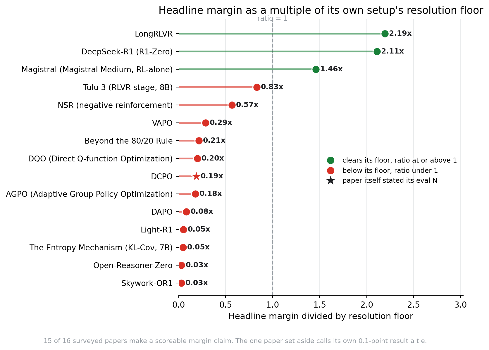
in our corpus whose headline is a single-benchmark margin. All 15 scoreable
claims could be scored, several only after digging the missing numbers out of
the papers’ own tables and code releases. 12 of the 15 margins are smaller
than what their own benchmark can reliably show. The median margin is a fifth
of its floor.</li>
  <li>The 3 margins that clear their floor tell one story between them. Two are
landslides from switching RL on at all, 46.8 and 55.4 points, big enough to
survive a 30-question benchmark. One is an ordinary-sized refinement that
clears because it was measured on 600 questions instead of 30. What separates
visible margins from invisible ones is how the margin compares to a floor the
benchmark’s size sets, not how impressive the method is.</li>
  <li>The same missing arithmetic appears upstream, where reward models, the graders
inside RL training, get chosen. All 6 public reward-model releases we audited
support “ours is better” with single point estimates. No seeds, no confidence
intervals, on the headline claim.</li>
  <li>Two failure mechanisms measured on real training runs show what that hides. A
reward model carrying half its real information fought the full-strength
version to an exact 108-to-108 draw on one of three otherwise-identical runs.
And the answer to which of two reward models looks better at a given training
checkpoint reversed sign up to 3 times over a run, with at most 1 of 6
checkpoint readings separating from zero.</li>
  <li>A comparison discipline that avoids both failure modes costs single-digit
dollars at the scale we ran it. Applied to our own two live reward-model
comparisons, it reads both as ties, and a length audit inside it showed that
one of our own strongest results was measuring response length, not reward
quality.</li>
</ul>

<h2 id="1-every-benchmark-has-a-smallest-gap-it-can-see-and-its-question-count-sets-it">1. Every benchmark has a smallest gap it can see, and its question count sets it</h2>

<p>A benchmark is a measuring instrument, and like any instrument it can only show
differences down to a certain size. A kitchen scale that reads in whole grams
cannot settle an argument about half a gram, and no amount of confidence in the
person doing the weighing changes that. For a benchmark, the smallest showable
difference is set by how many questions it has.</p>

<p>A benchmark score moves in steps of one question. On a 30-question test, each
question is worth 3.3 points, so the score cannot move in units finer than that.
The score also wobbles. Ask the same model the same 30 questions on another day,
with another sampling seed, and it will get a couple of questions right that it
missed before, and miss a couple it got right. That ordinary wobble moves a
30-question score by several points in either direction without anything about
the model changing. A real difference between two models has to be bigger than
the wobble before the test can show it reliably, where reliably means the test
would show it again on a second run.</p>

<p>Statistics has a standard tool for exactly this, built for drug trials and
opinion surveys. It is called the minimum detectable effect, and it is the
smallest true difference a test of a given size can be counted on to find.
Computing it takes two numbers, both usually printed in a paper: how many
questions the test has, N, and roughly how often the baseline gets them right,
p. Those two give the score’s natural wobble, and the convention multiplies that
wobble by 2.80. The 2.80 is two standard terms added together. The 1.96 keeps
the chance of a false alarm at 5 percent, and the 0.84 on top buys an 80
percent chance that a real gap of this size shows up again on a rerun.</p>

<div class="language-plaintext highlighter-rouge"><div class="highlight"><pre class="highlight"><code>smallest reliable gap = 2.80 x sqrt(2 p (1 - p) / N)
</code></pre></div></div>

<p>This paper calls that number the detection floor. It is a property of the test,
not of the models being tested.</p>

<p>The floor is a reliability bar, not a significance bar, and the two are
different heights because they are built from different pieces of that 2.80.
Significance asks whether the gap you measured once was probably not luck, and
that costs only the 1.96. The floor asks more, that a gap of this size would
also show up again on a second run, four times out of five, and that costs the
full 2.80. Dividing the two gives the point where the bars cross, 1.96 / 2.80
= 0.70. A margin at 70 percent of its floor sits exactly at the significance
bar. Between 70 percent and the full floor, both readings are true at once,
and this is the confusing zone worth naming plainly. A margin there is
significant on the run that produced it and still too small to count on seeing
twice. Below 70 percent it fails both bars. The floor is also easy to compute
for someone else’s result. It does not need their model, their code, or their
compute, only the two numbers already printed in their paper.</p>

<p>Now apply it to one real published result. DCPO reports beating its closest
baseline by 6.7 points on AIME24, from a baseline accuracy of 40 percent.
AIME24 has 30 questions, so p = 0.4 and N = 30, and the formula gives a floor
of 35.4 points. The reported margin is 6.7, which is 0.19 of the smallest gap
this test can reliably show. In question terms, the margin is about two
questions, on a test whose ordinary wobble is bigger than two questions.</p>

<p>That number does not say the margin is fake. The improvement may be real. It
says something narrower. The instrument that produced this number was never
capable of reliably showing a difference this small, so if the same comparison
were run again, the odds of seeing this margin again are poor, and that is true
even if the method genuinely works. From this test alone, there is no way to
tell a result like this apart from luck.</p>

<p>The rest of this paper does three things with that one idea. It runs the same
two-number check on every recent paper in our corpus that makes this kind of
claim. It looks at where reward models, the graders inside RL training, get
chosen, and finds the same arithmetic missing there. And it lays out a cheaper
way to run these comparisons, with what each step costs, including what that
way showed about two comparisons of our own.</p>

<h2 id="2-the-same-check-on-15-recent-papers-12-margins-are-below-their-own-floor">2. The same check on 15 recent papers: 12 margins are below their own floor</h2>

<p>Of 30 recent RL-for-reasoning papers in our corpus, 16 lead with a
single-benchmark margin rather than a cross-benchmark average or a ratio such
as a data-efficiency multiplier. One of the 16, REINFORCE++, is set aside for a
reason section 2.1 explains, and it is a reason in the paper’s favor. The other
15 could all be scored. For 10 of them the two needed numbers were stated
outright or settled by public knowledge of the benchmark, the way AIME24 is
known to have 30 questions and the GSM8K test set 1,319. For the other 5 the
numbers were recoverable with more digging, from the papers’ own results
tables, from an official code release, or from a benchmark’s released files,
and section 2.1 records where each recovered number came from. Nothing in this
table rests on a guess.</p>

<table>
  <thead>
    <tr>
      <th>Paper</th>
      <th>Benchmark</th>
      <th>Margin (pp)</th>
      <th>Baseline acc</th>
      <th>N</th>
      <th>N source</th>
      <th>Floor (pp)</th>
      <th>Margin / floor</th>
    </tr>
  </thead>
  <tbody>
    <tr>
      <td>LongRLVR</td>
      <td>RULER-QA (14B)</td>
      <td>15.73</td>
      <td>0.732</td>
      <td>600</td>
      <td>released predictions</td>
      <td>7.17</td>
      <td>2.19</td>
    </tr>
    <tr>
      <td>DeepSeek-R1</td>
      <td>AIME 2024</td>
      <td>55.4</td>
      <td>0.156</td>
      <td>30</td>
      <td>known</td>
      <td>26.25</td>
      <td>2.11</td>
    </tr>
    <tr>
      <td>Magistral</td>
      <td>AIME-24</td>
      <td>46.8</td>
      <td>0.268</td>
      <td>30</td>
      <td>known</td>
      <td>32.04</td>
      <td>1.46</td>
    </tr>
    <tr>
      <td>Tulu 3 (RLVR, 8B)</td>
      <td>GSM8K</td>
      <td>3.3</td>
      <td>0.843</td>
      <td>1,319</td>
      <td>known</td>
      <td>3.97</td>
      <td>0.83</td>
    </tr>
    <tr>
      <td>NSR</td>
      <td>MATH (Pass@256)</td>
      <td>0.6</td>
      <td>0.963</td>
      <td>5,000</td>
      <td>official eval config</td>
      <td>1.06</td>
      <td>0.57</td>
    </tr>
    <tr>
      <td>VAPO</td>
      <td>AIME 2024</td>
      <td>10.4</td>
      <td>0.500</td>
      <td>30</td>
      <td>known</td>
      <td>36.17</td>
      <td>0.29</td>
    </tr>
    <tr>
      <td>Beyond the 80/20 Rule</td>
      <td>AIME’24</td>
      <td>7.71</td>
      <td>0.558</td>
      <td>30</td>
      <td>known</td>
      <td>35.92</td>
      <td>0.21</td>
    </tr>
    <tr>
      <td>DQO</td>
      <td>GSM8K (greedy)</td>
      <td>1.05</td>
      <td>0.635</td>
      <td>1,319</td>
      <td>known</td>
      <td>5.25</td>
      <td>0.20</td>
    </tr>
    <tr>
      <td>DCPO</td>
      <td>AIME24</td>
      <td>6.7</td>
      <td>0.400</td>
      <td>30</td>
      <td>stated</td>
      <td>35.44</td>
      <td>0.19</td>
    </tr>
    <tr>
      <td>AGPO</td>
      <td>MATH-500</td>
      <td>1.4</td>
      <td>0.732</td>
      <td>500</td>
      <td>known</td>
      <td>7.85</td>
      <td>0.18</td>
    </tr>
    <tr>
      <td>DAPO</td>
      <td>AIME 2024</td>
      <td>3.0</td>
      <td>0.470</td>
      <td>30</td>
      <td>known</td>
      <td>36.10</td>
      <td>0.08</td>
    </tr>
    <tr>
      <td>Entropy Mechanism (KL-Cov, 7B)</td>
      <td>AIME24</td>
      <td>1.4</td>
      <td>0.212</td>
      <td>30</td>
      <td>known</td>
      <td>29.57</td>
      <td>0.05</td>
    </tr>
    <tr>
      <td>Light-R1</td>
      <td>AIME24</td>
      <td>1.7</td>
      <td>0.723</td>
      <td>30</td>
      <td>known</td>
      <td>32.37</td>
      <td>0.05</td>
    </tr>
    <tr>
      <td>Open-Reasoner-Zero</td>
      <td>AIME2024</td>
      <td>1.1</td>
      <td>0.470</td>
      <td>30</td>
      <td>known</td>
      <td>36.10</td>
      <td>0.03</td>
    </tr>
    <tr>
      <td>Skywork-OR1</td>
      <td>AIME24</td>
      <td>0.8</td>
      <td>0.814</td>
      <td>30</td>
      <td>known</td>
      <td>28.15</td>
      <td>0.03</td>
    </tr>
  </tbody>
</table>

<p><em>Floors are computed with the unrounded constant, 1.9600 + 0.8416 = 2.8016.
Section 1 shows 2.80 rounded for display. Margins follow one convention
throughout, the paper’s headline number against its closest baseline method.
For VAPO the table prints integers while its abstract carries the decimal, so
the margin is 10.4 against DAPO’s 50. Full-precision figures ship in the
companion repository, whose floor calculator recomputes every row and every
figure from the recorded inputs.</em></p>

<p><img src="/assets/images/writing/reward-shopping-audit/fig_margin_vs_floor.png" alt="Horizontal lollipop chart, headline margin divided by detection floor, one row per paper, sorted descending, with a ratio-equals-1 reference line. Three rows clear their floor: LongRLVR at 2.19, DeepSeek-R1 at 2.11, and Magistral at 1.46. Twelve rows sit below the line, from Tulu 3 at 0.83 down through NSR at 0.57, VAPO at 0.29, Beyond the 80/20 Rule at 0.21, DQO at 0.20, DCPO at 0.19, AGPO at 0.18, DAPO at 0.08, the Entropy Mechanism and Light-R1 at 0.05, and Open-Reasoner-Zero and Skywork-OR1 at 0.03." /></p>

<p>12 of the 15 margins sit below their own floor. The median margin is 0.20 of
its floor, a fifth of the smallest gap its own benchmark could reliably show.</p>

<p>The 3 rows that clear their floor say more together than any of them says
alone. DeepSeek-R1 and Magistral are landslides, 55.4 and 46.8 points, the
one-time leap from switching RL on at all. On a 30-question benchmark, where
floors run 26 to 36 points, only a landslide can clear. LongRLVR is the
opposite case and the more instructive one. Its 15.7-point margin is an
ordinary-sized refinement, one method improving on another, and it clears at
2.2 times its floor because its benchmark has 600 scored items, which puts the
floor at 7.2 points instead of 36. That reading survives a worst-case check.
If the benchmark’s three context lengths secretly reuse the same 200
underlying questions, the honest N drops to 200 and the ratio drops to 1.27,
still clear of its floor. So the dividing line in this table is not how
impressive the method is. It is whether the margin is large relative to a
floor the benchmark’s size sets. A big margin clears a small test, a modest
margin can clear a big test, and a small margin clears nothing. Size alone
rescues no one either. NSR was measured on 5,000 questions, the largest N in
the table, and still sits at 0.57 of its floor, because its margin over its
closest trained baseline is 0.6 points against a 1.1-point floor. One more
fact belongs to that row. At this metric the untrained base model scores 96.9,
the same as NSR itself, so the gain over the base model at this particular
endpoint is zero, and the 0.6 is its edge over PPO, not over doing nothing.</p>

<p>A margin computed from an averaged metric needs one caveat stated once. Most
AIME24 rows report an average over multiple sampled attempts per question,
written avg@32 or similar. Averaging over attempts shrinks the sampling part
of the wobble, so the true floor for those rows sits somewhat below the
computed one, bounded from below by how much questions genuinely differ. The
computed floors are therefore upper bounds and the ratios lower bounds, and
the caveat applies equally to every AIME24 row in the table, the old ones and
the recovered ones alike. It does not move any row across the line, because
the below-floor AIME24 rows sit at 0.29 of their floor or lower, and
question-to-question difficulty differences, which averaging cannot remove,
keep real AIME floors far above margins of a point or two.</p>

<p>The nearest prior statement of this problem is Hochlehnert et al.
(<a href="https://arxiv.org/abs/2504.07086">arXiv:2504.07086</a>), who make the small-benchmark argument for AIME directly
and first. Re-running released checkpoints under standardized decoding, they
find that one question moves pass@1 by 2.5 to 3.3 points on benchmarks of the
size they study, that pass@1 standard deviations across random seeds run as
high as 15 points on AIME’24, and that the improvements recent methods report
fall inside that variance. Ten of the fifteen rows above are AIME24 rows, so
their argument covers most of this table and the priority is theirs. Their
evidence needs a released checkpoint and the compute to re-run it. The
two-number check needs neither, which makes it available for releases with no
public checkpoint and for benchmarks nobody has re-evaluated.</p>

<h3 id="21-recovered-numbers-and-the-one-paper-set-aside">2.1 Recovered numbers, and the one paper set aside</h3>

<p>An earlier version of this census could score only 10 of the 16 papers and
excluded the rest for missing numbers. A challenge to go verify the exclusions
at the sources dissolved all of them, and the corrections belong on the
record. Three papers said to omit their baseline accuracy state it in their
own results tables. DQO’s table gives the DPO baseline at 63.46 percent
against its 64.51, exactly the 1.05-point margin its text claims. Beyond the
80/20 Rule’s table gives 55.83 against 63.54. VAPO’s abstract and table give
60.4 against DAPO’s 50. Two more needed the authors’ released artifacts
rather than the paper text. NSR’s “MATH” turns out to mean the full
5,000-question test set, settled by the dataset its official evaluation
script loads. LongRLVR’s evaluation size is 600 items, settled by the
prediction files shipped with its release, 100 per task per context length.
Recovering numbers this way cuts against the paper’s own convenience, since
every recovered row was a chance for the census pattern to break, and one
recovered row, LongRLVR, did break the earlier version’s cleanest
generalization and forced the size-sets-the-line reading above.</p>

<p>The one paper set aside is REINFORCE++, and it is set aside because it makes
no margin claim to score. Its own text reports 46.7 against GRPO’s 46.8 and
calls the result a tie, which is the correct reading of a 0.1-point gap on
that benchmark. One disclosure point still belongs here. The benchmark it
used, Arena-Hard-Auto, ships bootstrap confidence intervals in its standard
tooling, and the paper reports the scores without them. A reader deserves the
interval a benchmark’s own harness would have printed, most of all when the
honest conclusion is a tie. The paper also spans nine arXiv versions in which
this evaluation appears from the second year onward, so any citation of those
numbers should pin the version it read.</p>

<h3 id="22-the-other-number-nobody-reports">2.2 The other number nobody reports</h3>

<p>The floor needs N and p. An error bar needs a third number, how many training
seeds the headline run used and how much the result moved between them. A
companion census over the same 30-paper corpus checked for exactly that. One
of the 30 has no headline claim to score, Kimi K2 (<a href="https://arxiv.org/abs/2507.20534">arXiv:2507.20534</a>), which
reports overall model capability against other released models rather than a
method-versus-baseline comparison. Of the 29 that remain, 27 report no
training-seed count at all for their headline result, 93 percent of the
corpus, and only 2 pair a seed count with its own between-seed spread. Put
the two censuses together and a reader of this literature usually cannot
reconstruct an error bar in either direction, not across questions, because N
goes unstated, and not across runs, because the seeds do. That is a statement
about what the documents contain, not about anyone’s intent.</p>

<h2 id="3-the-models-grading-your-training-are-chosen-the-same-blind-way-6-of-6-releases-one-number-no-error-bars">3. The models grading your training are chosen the same blind way: 6 of 6 releases, one number, no error bars</h2>

<p>The check so far scores papers about training methods. The same question can be
asked one level up. Reward models, the trained graders that steer RL training
wherever no automatic checker exists, are themselves compared, ranked, and
chosen, and the release documents that support those choices can be read with
the same two questions in mind. How many runs, and where is the error bar.</p>

<p>We read the evaluation sections of six public reward-model releases from 2024
and 2025: Skywork-Reward-V2, the Tulu/RewardBench 2 line, GRM,
Nemotron-4-340B-Reward with HelpSteer2, ArmoRM, and INF-ORM-Llama3.1-70B. For
each we recorded which benchmarks it reports, how many seeds, what training
horizon, and whether variance or a confidence interval appears anywhere near
the headline number.</p>

<table>
  <thead>
    <tr>
      <th>Release</th>
      <th>Headline practice</th>
      <th>Downstream (RLHF/BoN) validation</th>
      <th>Seeds reported</th>
      <th>Variance/CI reported</th>
    </tr>
  </thead>
  <tbody>
    <tr>
      <td>Skywork-Reward-V2 (<a href="https://arxiv.org/abs/2507.01352">arXiv:2507.01352</a>)</td>
      <td>7 to 8 benchmarks, point estimates</td>
      <td>Best-of-N only. No full RLHF run in main text</td>
      <td>None</td>
      <td>No. A 0.6-point ablation spread exists, unattached to the leaderboard claim</td>
    </tr>
    <tr>
      <td>AI2 Tulu / RewardBench 2 (<a href="https://arxiv.org/abs/2506.01937">arXiv:2506.01937</a>)</td>
      <td>RewardBench 2, 6 domains, point estimates</td>
      <td>Most extensive. 113 best-of-N, 17 PPO vs Tulu 3</td>
      <td>None stated per configuration</td>
      <td>No, but one saturation caveat volunteered (quoted below)</td>
    </tr>
    <tr>
      <td>GRM (<a href="https://arxiv.org/abs/2406.10216">arXiv:2406.10216</a>)</td>
      <td>RewardBench + 2 out-of-distribution sets, point estimates</td>
      <td>Yes. Full PPO trajectory vs. gemma-2b-it</td>
      <td>1 per trajectory</td>
      <td>No confidence bands on the curves</td>
    </tr>
    <tr>
      <td>Nemotron-4-340B-Reward / HelpSteer2 (<a href="https://arxiv.org/abs/2406.11704">arXiv:2406.11704</a> / <a href="https://arxiv.org/abs/2406.08673">2406.08673</a>)</td>
      <td>RewardBench only, overall plus per-category scores, all point estimates</td>
      <td>None isolated</td>
      <td>None</td>
      <td>No</td>
    </tr>
    <tr>
      <td>ArmoRM (<a href="https://arxiv.org/abs/2406.12845">arXiv:2406.12845</a>)</td>
      <td>RewardBench only, overall plus per-category scores, all point estimates</td>
      <td>None</td>
      <td>None</td>
      <td>No</td>
    </tr>
    <tr>
      <td>INF-ORM-Llama3.1-70B (HuggingFace model card)</td>
      <td>RewardBench only, single dated-snapshot number</td>
      <td>None</td>
      <td>None</td>
      <td>No</td>
    </tr>
  </tbody>
</table>

<p>Across all six, the pattern is one pattern. Every release supports its “ours
is better” claim with point-estimate scores on a static benchmark, headlined
by a single overall number, and none reports a standard deviation, a
confidence interval, or a multi-seed replication for that headline number.
Several break the benchmark out by category, which is more disclosure than a
bare overall score and is still more point estimates rather than an error
bar. Where a lab’s own data does surface run-to-run variation, the variation
stays out of the headline. Skywork’s own ablation measures a 0.6-point spread
across data subsets and never attaches it to the seven-benchmark leaderboard
table. ArmoRM calls its 0.3-point gap over Nemotron-4-340B-Reward “nearly on
par” with no uncertainty estimate in either direction, and those two numbers
sit closer together than any variance either lab discloses for its own
measurement.</p>

<p>Downstream validation, actually training a policy with the reward model and
looking at what comes out, is rare, and where it exists it is real. AI2
trains and evaluates 113 best-of-N and 17 PPO configurations against actual
Tulu 3 policies. GRM plots reward divergence across a full PPO training
horizon. Both engage with the downstream question in a way the other four
papers do not attempt. Nemotron-4-340B-Reward is not separately validated at
all. Its reward model is folded into a training pipeline and judged only
through the trained policy’s aggregate scores.</p>

<p>AI2’s disclosure goes furthest, and one sentence of it deserves quoting in
full, because it is the only place across the six releases where a lab
volunteers that its own evidence may not distinguish between the reward
models its leaderboard ranks:</p>

<blockquote>
  <p>“PPO performance quickly saturates to a similarly good performance matching that of Tulu 3
8B DPO for all decent-to-good reward models whose RewardBench 2 scores range from 49.8 to
68.5.”</p>
</blockquote>

<p>Read plainly, that sentence says downstream policy quality stops responding
to reward-model differences above some quality bar, which would mean the
leaderboard differences among good reward models are not the thing driving
downstream outcomes. Even this, the cleanest practice of the six, states no
seed counts per configuration and picks its reported checkpoint after the
fact rather than fixing a horizon in advance. GRM earns credit for a
different reason. It is the only release that treats the training horizon as
an object of study, plotting a whole trajectory rather than an endpoint, and
it does so from a single seed. The one paper that shows a trajectory at all
is also the clearest illustration of why seed count and horizon need
attention together. Section 4 measures exactly that, with real training runs
and real reward models.</p>

<h2 id="4-two-ways-a-cheap-comparison-lies-an-unlucky-seed-can-erase-a-real-gap-and-an-early-reading-does-not-predict-the-end">4. Two ways a cheap comparison lies: an unlucky seed can erase a real gap, and an early reading does not predict the end</h2>

<p>Two training runs can differ for three mundane reasons before any interesting
one: the data order the seed sets, the weight initialization, and the random
draws behind each sampled rollout. A gap between two runs says nothing about
the thing being compared until all three are ruled out. The seed-masking runs
below rule out all three between the compared variants. Both variants draw
their per-token sampling randomness from the same keyed noise stream, replayed
bit for bit, so at the first training step both variants sample identical
token sequences, checked directly on the machine before any scored run
launched. From that point on, a gap between them has one remaining
explanation, the reward signal. The horizon-flip runs are different and the
difference limits how hard they can be read. They were trained earlier in
this project, before that coupling existed, and the question asked of them is
not which variant won but whether an early reading points the same way the
converged reading does, both taken from the same recorded histories.</p>

<h3 id="an-unlucky-seed-can-erase-a-real-known-difference">An unlucky seed can erase a real, known difference</h3>

<p>We built a reward model that is measurably worse than a real one, rather than
guessing at how a weak model would behave. It blends GRM-Gemma2-2.6B’s own
scores half-and-half with a within-group shuffled copy of themselves, which
destroys half the information while keeping the score’s scale and texture.
This half-signal variant trained against the full-strength GRM as the other
variant, across three training seeds, judged blind on held-out prompts by two
reward models that trained neither variant. The ground truth is known by
construction. The full-strength variant should win, because half the signal
it carries was deliberately destroyed in the other.</p>

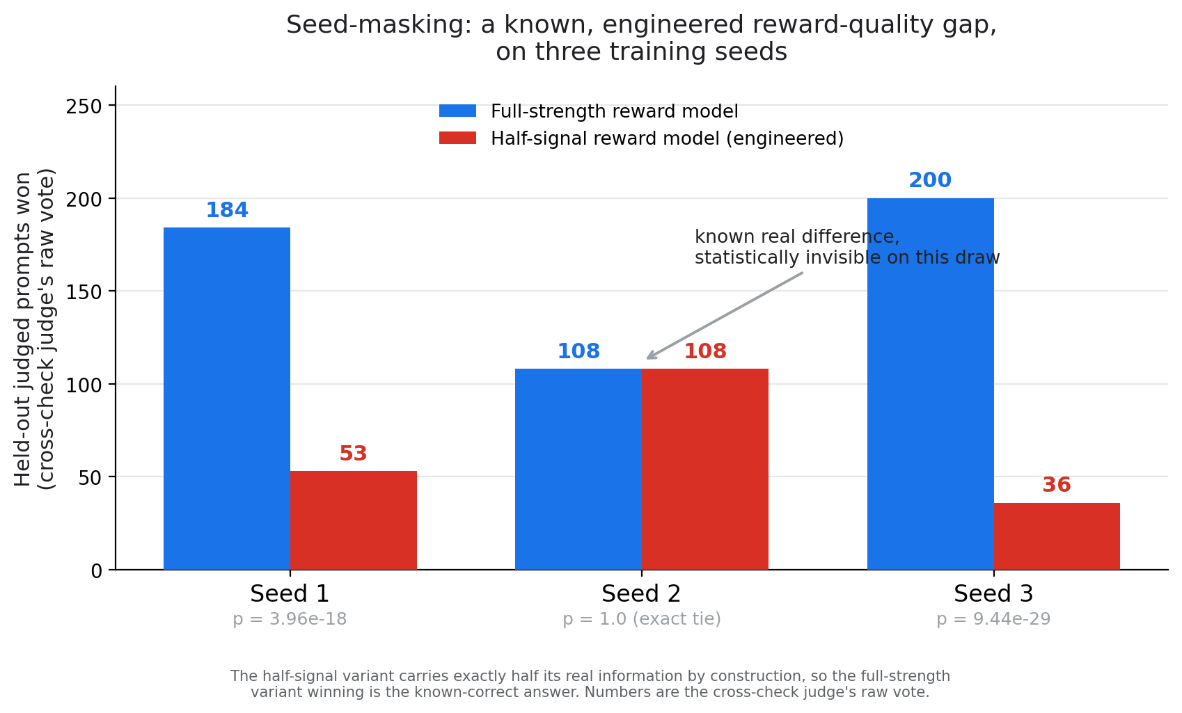
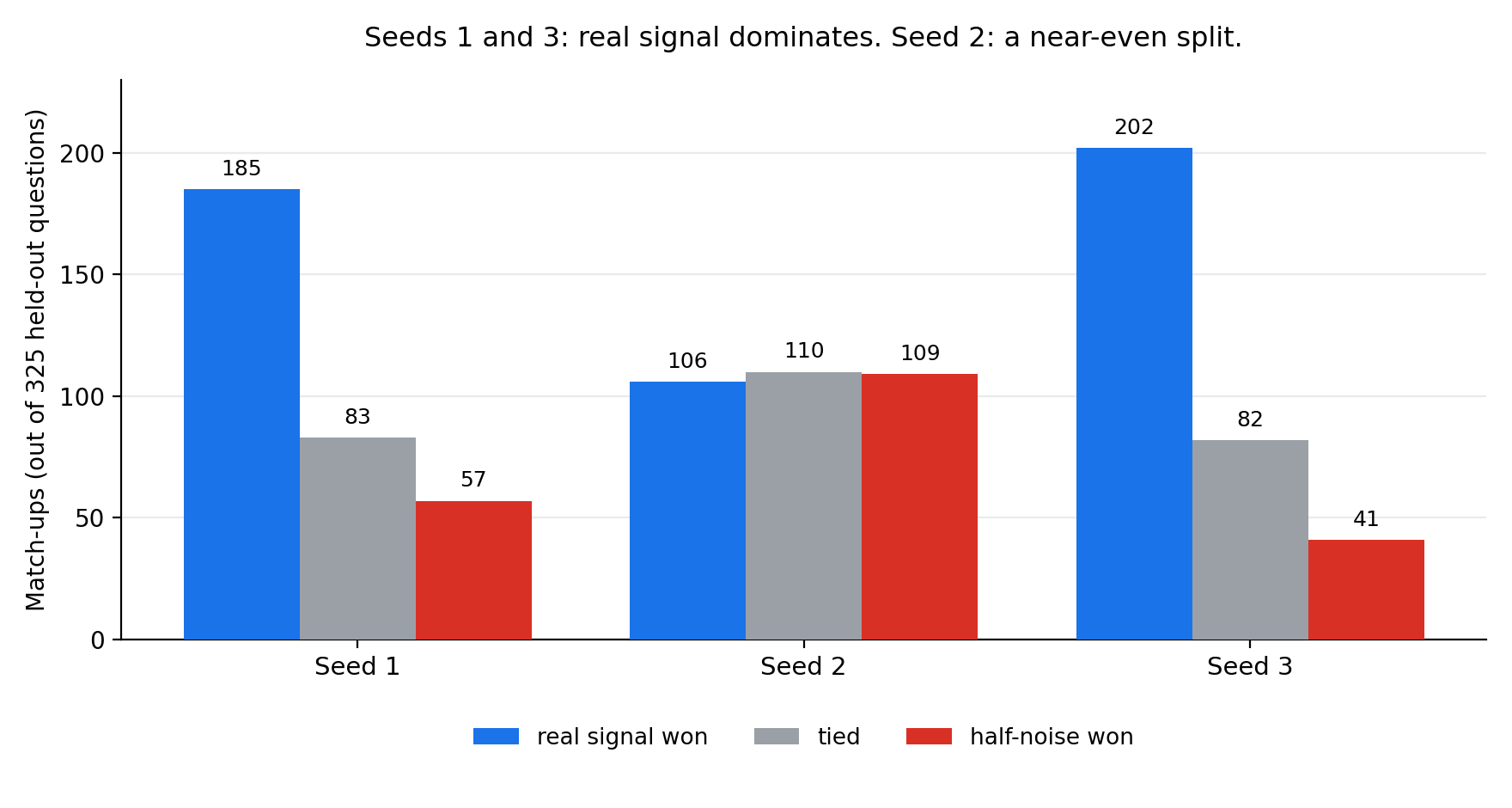
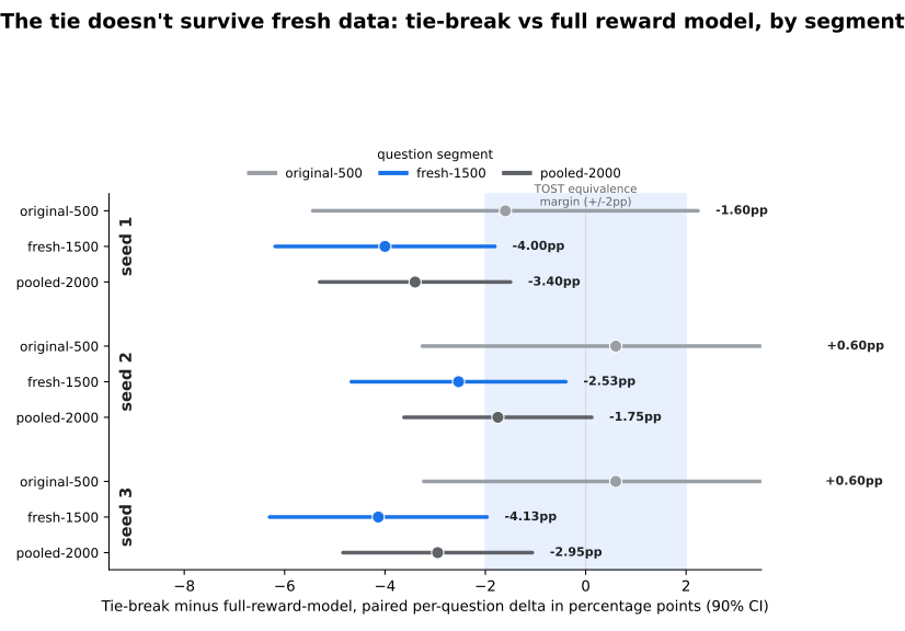
<p><img src="/assets/images/writing/reward-shopping-audit/fig1_seed_masking.png" alt="Grouped bar chart, three training seeds. Seed 1: full-strength reward model 184 wins to half-signal reward model's 53 (p = 3.96e-18). Seed 2: 108 wins to 108 wins, an exact tie (p = 1.0), annotated &quot;known real difference, statistically invisible on this draw.&quot; Seed 3: 200 wins to 36 (p = 9.44e-29). All bars are the cross-check judge's raw vote." /></p>

<p>Two of the three seeds detect the difference overwhelmingly. Under the raw
judge vote, seed 1 favors the full-strength variant 184 wins to 53, at p =
3.96 x 10⁻¹⁸ on the Mistral judge. Seed 3 favors it 200 to 36 on the same
judge, at p = 9.44 x 10⁻²⁹, and 202 to 41 on the other. Seed 2 shows nothing
at all. One judge’s tally lands at exactly 108 wins apiece, a dead heat, p =
1.0. The other judge reads the same seed 106 to 109, leaning the wrong way.
This is an engineered, known information deficit, and on this one seed
neither of two independent judges can see it even at the level of raw
preference counts. Under the length-corrected primary scoring rule that
section 5 introduces, the picture does not improve. Seed 2 is the one seed
whose sign flips against the other two on both judges. The pooled reading
across all three seeds stays significant in the correct direction, at p =
0.008 to 0.003 depending on judge, and the seeds do not all agree with it,
so under the two-part rule defined in section 5 no winner is called.</p>

<p>The instrument is not blind. Two of three seeds detected a half-strength
reward model at significance levels that would be extraordinary in most
empirical settings. The finding is narrower and worse for common practice. A
single training seed is not a reliable unit of evidence for a reward-model
comparison, because the seed-to-seed variance in how a comparison plays out
is large enough for one unlucky draw to erase a real, substantial, known
difference. A lab that reports “we compared reward model A to reward model B
and A won,” the practice every release in section 3 follows, has a meaningful
chance of reporting a property of its seed rather than a property of the two
reward models, and which seed a lab happened to run is not disclosed in any
of the six releases.</p>

<h3 id="an-early-reading-does-not-reliably-predict-where-a-run-ends-up">An early reading does not reliably predict where a run ends up</h3>

<p>The training horizon is a second, independent axis on which a single reading
can mislead. We used recorded evaluation histories from three training
variants on a checkable task, three seeds each, with a real early-stopping
rule, so that “converged” and “peak” are both well-defined per run. The
variants are a checker-only variant, rewarded by GRPO’s binary right/wrong
verifier, a full-reward-model variant, rewarded by a dense reward model on
every rollout, and a localized-reward-model variant that applies the dense
model only to break ties the checker cannot. The question asked is
descriptive. If a comparison between two variants had been read at an
intermediate checkpoint, would it point the same way the converged reading
does. The converged reading is itself a point estimate rather than a ground
truth, and the one converged comparison that was properly tested reads as a
statistical tie at p = 0.33, so agreement here means two point estimates
sharing a sign, nothing stronger.</p>

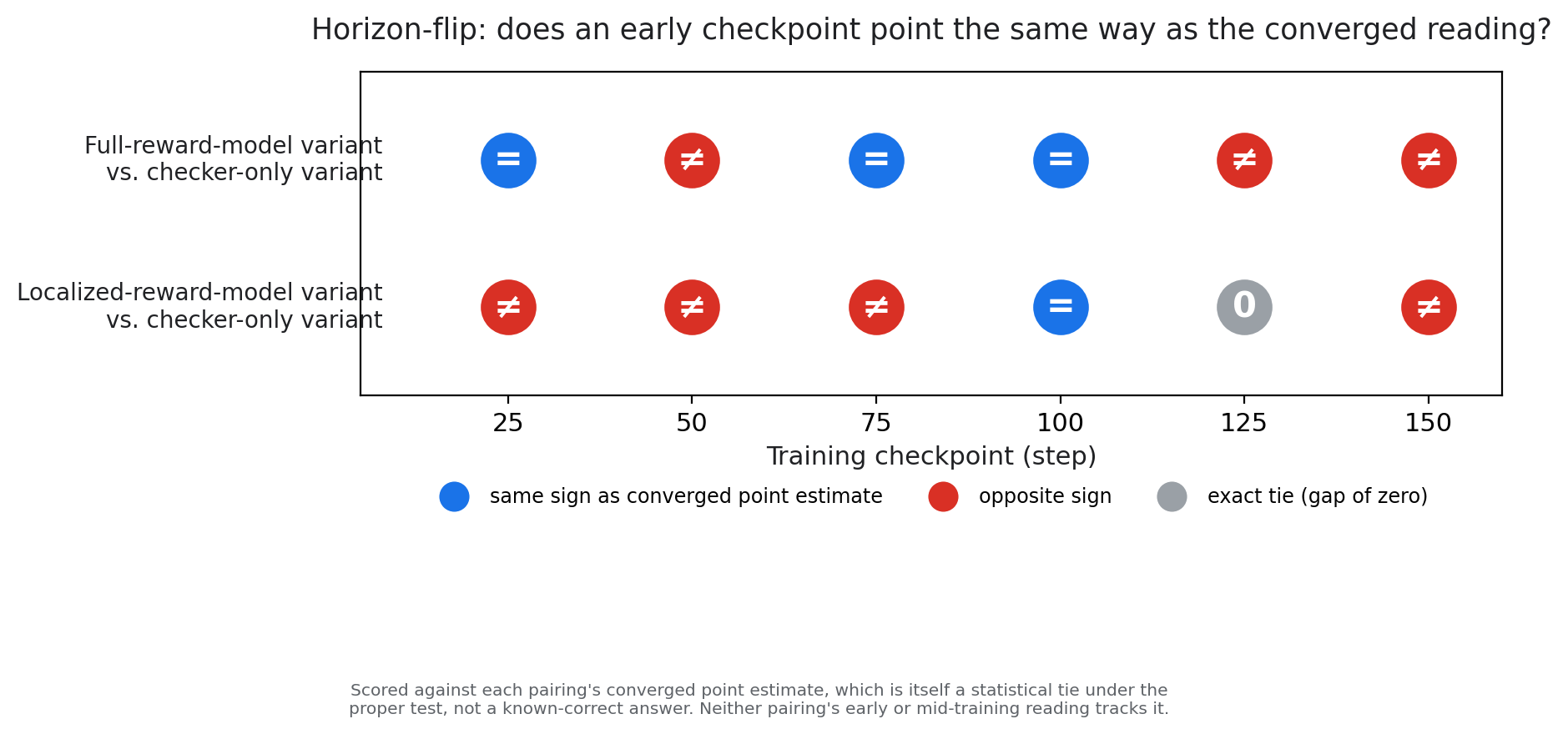
<p><img src="/assets/images/writing/reward-shopping-audit/fig2_horizon_flip.png" alt="Two rows of six markers, one marker per training checkpoint from step 25 to step 150. Each marker scores whether that checkpoint's reading has the same sign as the same pairing's converged point estimate, which is itself a tie under the proper test rather than a known correct answer. The top row shows the full-reward-model variant against the checker-only variant. It matches the converged sign at steps 25, 75, and 100, and takes the opposite sign at steps 50, 125, and 150. The bottom row shows the localized-reward-model variant against the checker-only variant. It takes the opposite sign at steps 25, 50, 75, and 150, lands on an exact tie at step 125, and matches at step 100." /></p>

<p>Across six checkpoints spanning steps 25 through 150, the answer is no for
two of the three pairings. The full-reward-model variant against the
checker-only variant flips sign three times across the six checkpoints and
never settles into the direction it eventually converges to. The point
estimates show the full-reward-model variant with a transient mid-training
lead of 1.8 to 3.8 points across the three seeds, read at each variant’s own
peak. That lead does not clear the rule, landing at p = 0.196 pooled under the same
rule used everywhere else in this paper. By convergence the point estimates
lean the other way, and the three seeds split in sign. The
localized-reward-model variant against the checker-only variant matches its
converged sign at exactly one of the six checkpoints, on a gap of 0.13
points, too small to separate from zero. The third pairing, localized
against full, is the one that partly settles. It lands on the converged side
at three of six checkpoints including both of the last two, and it still
points the wrong way at three of the first four.</p>

<p>A follow-up interval analysis on the same histories makes the practical
reading blunter. With a 95 percent confidence interval on each checkpoint
comparison, at most one of the six checkpoints in the window separates from
zero for any pairing, and no pairing shows two significant readings with
opposite signs. The sign flips are point estimates wobbling inside their own
intervals. That hardens the finding rather than softening it. A pilot
reading a single checkpoint in this window is not reading an unstable truth.
It is reading noise that happens to wear a sign. The one checkpoint that
does separate cleanly is also the most misleading one. At step 150, pooled
across seeds, the full-reward-model variant leads by 2.9 points, interval
0.4 to 5.5. By convergence that lead is gone, and the properly tested
endpoint comparison is a tie.</p>

<p>One tempting fix does not work. Reading a summary of the trajectory up to a
horizon, rather than a single point on it, was tested directly against the
same data. The best of four trajectory summaries tried, a linear slope over
recent checkpoints, beats a plain point-in-time reading in exactly one of
fifteen pair-by-horizon comparisons, which is not an improvement at that
sample size. A cumulative running average gets the eventual winner’s sign
wrong at all fifteen, for a diagnosable reason. It systematically punishes a
variant that starts slowest and finishes best, which is exactly the variant
that wins this comparison. If truncating a run early creates this much risk,
the fix is not a cleverer way to read a truncated run. It is not truncating
it, and that choice is where the next section starts.</p>

<h2 id="5-the-fix-costs-single-digit-dollars-six-steps-each-with-its-cost">5. The fix costs single-digit dollars: six steps, each with its cost</h2>

<p>If a single seed and a single horizon are each independently unreliable, the
response is not a cleverer way to read one seed at one horizon. It is a
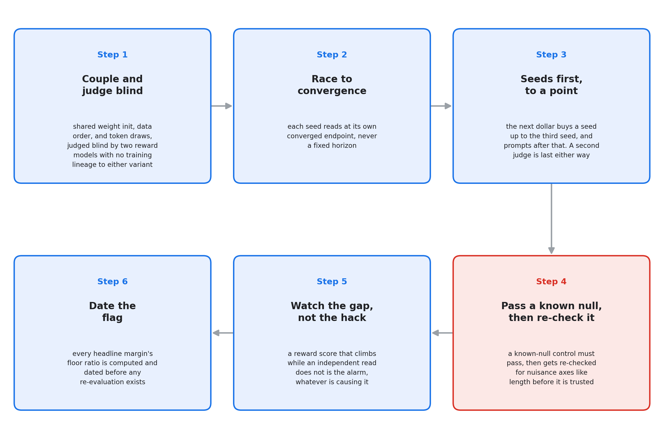
design that does not depend on either being reliable alone. That design
follows, as six numbered steps with what each one costs.</p>

<p><img src="/assets/images/writing/reward-shopping-audit/fig6_protocol_pipeline.png" alt="Six-box pipeline diagram in a two-row grid. Top row, left to right: Step 1, Couple and judge blind. Step 2, Race to convergence. Step 3, Seeds first, to a point. An arrow drops from Step 3 straight down to Step 4, positioned below it in the bottom row. Bottom row, right to left, continuing the flow: Step 4, Pass a known null, then re-check it, shown in red as the one step whose first pass was revised after a length confound. Step 5, Watch the gap, not the hack. Step 6, Date the flag, on the far left. Reading the bottom row right to left keeps the sequence 4 to 5 to 6 unbroken." /></p>

<table>
  <thead>
    <tr>
      <th>Step</th>
      <th>What it does</th>
      <th>What it costs</th>
    </tr>
  </thead>
  <tbody>
    <tr>
      <td>1. Couple and judge blind</td>
      <td>Two training variants share weight init, data order, and (until they diverge) token draws. Judged blind by two reward models with no training lineage to either variant.</td>
      <td>About $13 to $29 per live comparison, training and blind judging together</td>
    </tr>
    <tr>
      <td>2. Race to convergence</td>
      <td>Each seed reads at its own converged endpoint, never a fixed horizon.</td>
      <td>Nothing beyond step 1. It is a stopping-rule choice</td>
    </tr>
    <tr>
      <td>3. Seeds first, to a point</td>
      <td>The next dollar buys a seed up to the third seed, and evaluation prompts after that. A second judge comes last under either goal.</td>
      <td>$3.50 per seed, $0.50 per 100 prompts, $0.30 for a second judge</td>
    </tr>
    <tr>
      <td>4. Pass a known null, then re-check it</td>
      <td>A known-null control must pass, and then gets re-checked for nuisance axes like length before it is trusted.</td>
      <td>$19.39 for the plant control, $0 for the re-analysis</td>
    </tr>
    <tr>
      <td>5. Watch the gap, not the hack</td>
      <td>A reward score that climbs while an independent read does not is the alarm, whatever is causing it.</td>
      <td>$0, a re-analysis of already-recorded drift data</td>
    </tr>
    <tr>
      <td>6. Date the flag</td>
      <td>Every headline margin’s floor ratio (section 2) is computed and dated before any re-evaluation exists, then scored against whatever lands later.</td>
      <td>$0, reading only</td>
    </tr>
  </tbody>
</table>

<p><strong>Step 1: couple two training variants and judge them blind.</strong> The task is
the non-verifiable slice of an instruction dataset, prompts with no checkable
answer, 4,666 items at a pinned revision. One deterministic construction,
fixed before any run, takes 500 items as the training pool and a disjoint
block as the held-out evaluation pool. The first live comparison in section 6
read on a 200-item evaluation pool. The second read on a 325-item pool built
by the same construction with a larger cut, whose first 200 items are
byte-identical to the earlier pool. The policy is Qwen2.5-1.5B-Instruct,
trained by LoRA under GRPO with eight rollouts per prompt. Within a training
seed, the two compared variants share the same adapter initialization and the
same per-step data order, and both variants’ token sampling is driven by the
same fixed pseudo-random draw, computed per prompt, step, sample, and decode
position. The trick is borrowed from communication-free noise coupling built
for speculative decoding (Daliri, Musco, and Suresh, <a href="https://arxiv.org/abs/2408.07978">arXiv:2408.07978</a>). At
the first training step, before the weights have diverged, the two variants’
sampled token sequences are bit-for-bit identical, checked directly on the
machine. Any difference downstream of step one is attributable to the
reward, not to rollout luck.</p>

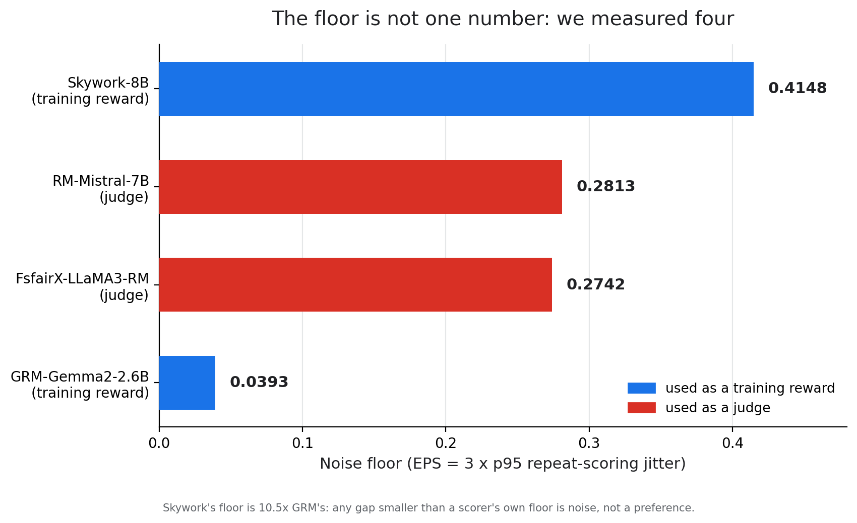
<p>Before training, all four scoring models in the pipeline, the two reward
models being compared and the two judges, are measured for their own
repeat-scoring noise. Each of 64 held-out items is scored five times, and 3
times the 95th-percentile spread across those scorings becomes that scorer’s
noise floor. GRM-Gemma2-2.6B’s floor is 0.0393. Skywork-8B’s is 0.415, 10.5
times larger. The two judges land at 0.274 and 0.281. Any score gap smaller
than a scorer’s own floor is treated as a tie everywhere downstream. Two
notes belong to that measurement. The 3x multiplier is a disclosed design
constant written into the spec before any floor was measured, deliberately
generous so the band errs toward calling a real difference a tie. And a
reward model is a deterministic function of its input, so a spread across
repeat scorings of the same text needs a mechanism. The mechanism is batch
composition. The five scorings differ only in what else shares the batch,
and changing the batch changes its padded shape and the order in which
floating-point additions happen on the accelerator. Those additions are not
associative, so the same text scored beside different neighbors comes back
with slightly different scores. This is the known explanation for the
effect, not something this project discovered. The protocol measures its
size by scoring each item alone and then at four positions inside an
eight-sequence batch.</p>

<p>At read time, both variants generate greedy responses on the held-out
prompts, pooled with the untrained baseline’s own responses, shuffled, and
scored by two reward models that trained neither variant and share no
training lineage with either one, the contamination risk Preference Leakage
names directly (<a href="https://arxiv.org/abs/2502.01534">arXiv:2502.01534</a>). Variant identity is never shown to either
judge. One judge is primary and the other is a cross-check, and a result the
cross-check disagrees with is reported as a disagreement, not a finding. The
verdict rule works on prompts, not scores. Within a seed, a prompt counts as
a win for whichever variant its judge scored higher, unless the two scores
fall inside the judge’s own floor, in which case the prompt is a tie and
drops out. Each prompt then votes once, by majority across the seeds. Two
conditions must hold together for a comparison to count as a called win. The pooled
per-prompt majority vote must be significant on an exact two-sided binomial
test, and every seed’s own sign must agree with the majority. That pair of
conditions is the two-part rule, and every result in this paper is held
to it. Section 4’s seed-masking result shows the two conditions doing their
jobs. The pooled vote there is significant at p = 0.008, so the first
condition is met, and seed 2’s own sign points against the majority, so the
second fails and no winner is called.</p>

<p><strong>Step 2: race each variant to its own convergence, never a fixed horizon.</strong>
The horizon findings in section 4 force this choice. Each seed reads at its
own converged endpoint, whatever the step count. Running the comparison
small already saves roughly 50 times the parameters of a production
fine-tune. Stopping early would save a further 2.5 times and is exactly
where the horizon risk lives, so this design gives that discount back. A
worked check on the section 4 data shows the stakes, using the same three
variants. Reading the three seeds’ endpoints on 2,000 questions, the
full-reward-model variant and the checker-only variant are statistically
tied, p = 0.33 pooled. Reading them at a shared mid-training checkpoint on
the original 500 questions instead, the full-reward-model variant leads by
2.0 to 4.6 points at pooled p = 0.025, a lead it gives back by convergence.
Selecting a checkpoint by validation accuracy on the original 500, a rule
fixed before 1,500 fresh questions were scored, and then reading only the
fresh 1,500, the full-reward-model variant wins 211 of 365 separating
questions at pooled p = 0.0033, all three seeds agreeing. Reading each
variant’s final, unselected checkpoint on the same fresh 1,500 instead, it
trails by 0.8 to 1.3 points with all three seeds agreeing on the losing
side, p = 0.36. Same runs, four defensible readings, three different
stories. On a checkable task the checker itself finds the peak for free. On
a task with no checker, nothing that cheap exists, because the reward
model’s own training score keeps climbing after real accuracy has turned
over, so finding the peak needs a second, independent signal, and paying
for that signal is the expense a reward model was supposed to remove.</p>

<p><strong>Step 3: spend the next dollar on a seed, up to the third seed, and on
prompts after that.</strong> The pooled verdict’s uncertainty splits into three
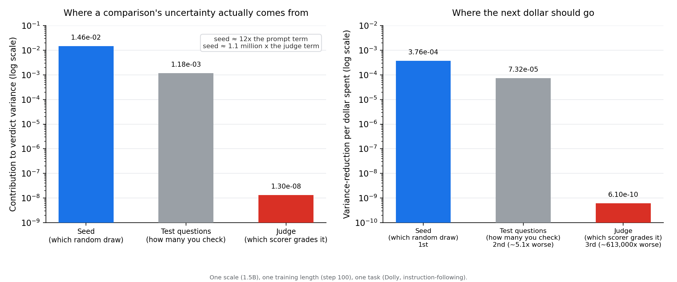
measured parts, seed-to-seed variation, per-prompt sampling noise, and
judge-scoring jitter. Across four independent readings of that split, the
seed part runs roughly 4 to 30 times larger than the prompt part and orders
of magnitude larger than the judge part. The judge part is small partly
because the two judges are not very independent. Their score differences
correlate at r = 0.91 to 0.92, which makes two judges count as about 1.05
independent opinions, and it means the cross-check this protocol leans on is
weaker corroboration than “two judges agreed” sounds. In money, one more
training seed costs about $3.50 at this scale and buys roughly 5 times the
uncertainty reduction that $0.50 of additional prompts buys. A second
cross-check judge costs about $0.30 and buys almost nothing, for the same
correlation reason.</p>

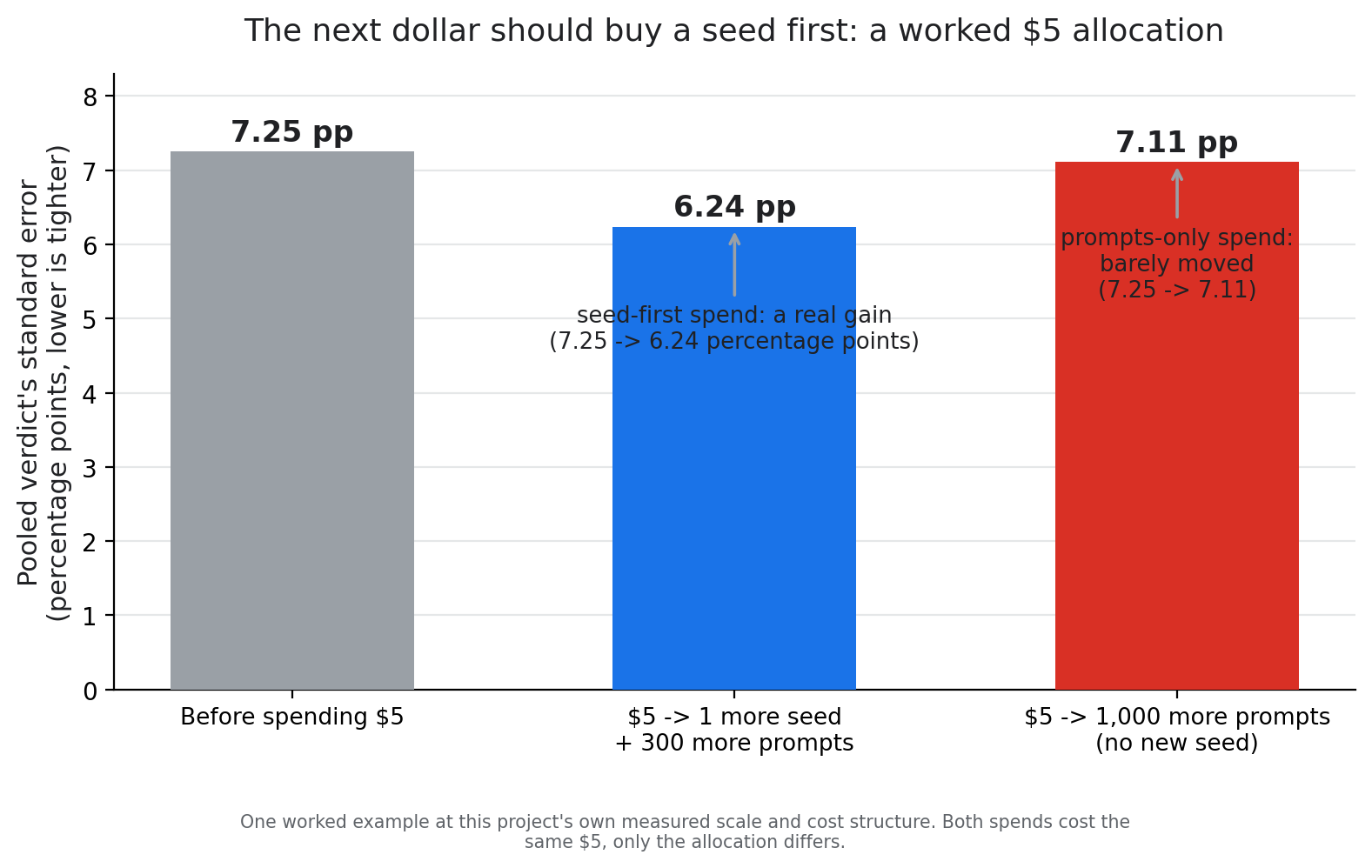
<p><img src="/assets/images/writing/reward-shopping-audit/fig3_seeds_first_budget.png" alt="Bar chart, three bars. Before spending the $5, the pooled verdict's standard error is 7.25 percentage points. Spending the $5 on one more seed plus 300 more prompts tightens it to 6.24 percentage points. Spending the same $5 entirely on 1,000 more prompts, with no new seed, leaves it at 7.11 percentage points, barely moved." /></p>

<p>A worked $5 split makes it concrete. One more seed plus 300 more prompts
tightens the pooled standard error from 7.25 to 6.24 percentage points. The
same $5 spent entirely on 1,000 more prompts leaves it at 7.11, barely
moved. The rule has two regimes, and stating it as “seeds before everything”
would misdescribe this project’s own numbers. While a comparison runs on one
or two seeds, the next dollar buys a seed, because the seed term dominates
and nothing else touches it. At three seeds the seed term stops paying.
Under the two-part rule, each added seed sharpens the pooled test and
simultaneously adds one more chance for a seed to point the other way, and
the two effects roughly cancel. The smallest win-rate gap the rule
reliably catches is 8.7 percentage points at 3 seeds and still 8.2 at 5, while doubling
the per-seed prompt count moves the same floor from 8.7 to 6.1. Seeds up to
three to know where you stand, prompts after that to nail down what you
found, and a second judge last under either goal, at this project’s own
measured scale. One honest boundary. This ranking counts a second judge
only for noise reduction, not for its separate value in catching a shared
bias or contamination that a single judge cannot see by construction, and
step 5 shows a concrete case of that separate value. A projection of this
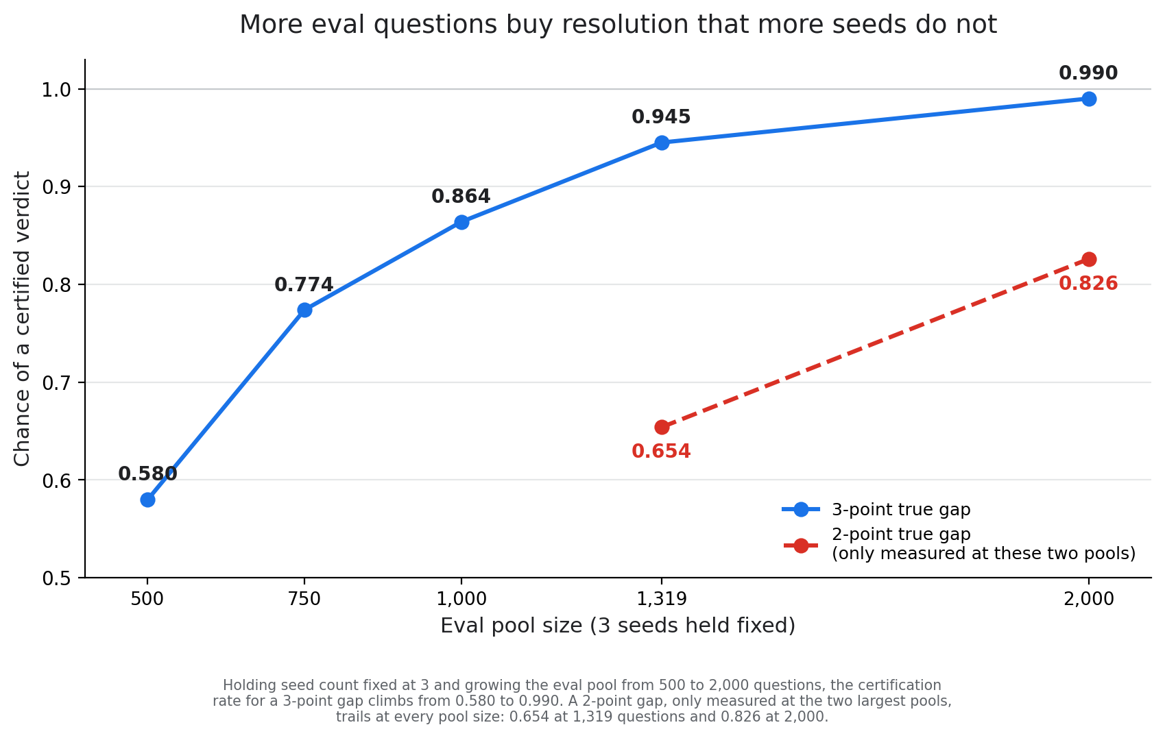
arithmetic was also written down and dated before the 1,500 extra questions
above were bought, at 0.990 for a 3-point gap and 0.833 for 2 points. The
realized numbers came out at 0.990 and 0.826.</p>

<p><strong>Step 4: pass a known-null control, then check what the passing grade is
measuring.</strong> Two controls ran against the verdict machinery
before any live comparison. A positive control confirmed the judges detect a
known, large effect, each trained checkpoint against the untrained starting
policy, and it cleared all six pairings tested at primary-judge p-values
from 2.6 x 10⁻³² to 3.3 x 10⁻²². A plant control replaced one variant’s
reward with a permutation of its own scores, which carries zero usable
information by construction, and the judges caught it just as decisively.
The pooled vote favored the honestly-scored variant 143 to 21 across 164
decided prompts, p = 1.7 x 10⁻²³, with the cross-check judge agreeing at 152
to 19, p = 5.9 x 10⁻²⁷. One note on these p-values. The code that first
computed them used an absolute floating-point tolerance that floored any
result below about 10⁻¹⁵, so the stored outputs understated how extreme the
strongest tests were. The counts are unaffected, and the values printed
here are recomputed exactly.</p>

<p>Then the passing grade itself got checked, and this is where the protocol
caught one of its own results. A practitioner’s instinct says reward models
reward length, a bias documented for LLM judges generally (Zheng et al.,
<a href="https://arxiv.org/abs/2306.05685">arXiv:2306.05685</a>), and the instinct turned out substantially right. The
honestly-scored variant’s responses grow to a mean of 121 to 134 tokens by
read time while the plant-scored variant’s stay near 70, and both judges
carry a length-correlated scoring bias of similar size, r of roughly 0.36
to 0.47. Restricting the plant control to response pairs of matched length
collapses the result. At a 20 percent length band the vote no longer clears
significance, p = 0.418, down from 10⁻²³, on 38 decided prompts. At the
tightest band the direction reverses on 21 prompts, with about 86 percent
of pairs discarded by the matching, a weak reading on a small slice rather
than a finding. A regression that keeps every pair says the same thing more
precisely. Length alone explains 40 percent of the score-difference
variance, and the length-independent remainder is 0.309, standard error
0.086, which sits barely above the judges’ own noise floor of 0.274. A
result that stood 21 to 25 orders of magnitude past significance survives,
once length is accounted for, only as a small, barely-above-floor residual.</p>

<p>Regressing length out is not automatically safe either, and this is the
part that stops the fix from being a reflex. On three settings with
checkable correctness, the reward model audited showed no positive length
preference at fixed correctness, and residualizing anyway hurt
truth-agreement in two of them, by 0.8 and 3.0 points overall and by 10.3
points in the worst condition, because in those settings short answers are
more often right, so subtracting length subtracts real signal. The rule
this forces: measure a judge’s length slope at fixed quality wherever a
checker makes that possible, and residualize only where the slope is
positive. Where no checker exists the slope is a disclosed, unverifiable
quantity, not a license to residualize by default. This rule was written
after the first of section 6’s two live comparisons had already run, so
only the second was scored under it from the start, and the same
length-driven mechanism turns out to explain the one anomalous seed in the
first comparison. Whenever a judge’s score tracks some axis that is not the
thing being measured, any drift between two variants along that axis gets
converted into what looks like reward-quality signal. We call this
nuisance-axis amplification, and it is the reading most consistent with
two single-instance findings rather than an independently proven mechanism.</p>

<p><strong>Step 5: watch for a reward score that climbs while an independent read
does not.</strong> Nobody needs to identify which failure mode a reward model has
fallen into before being warned something is wrong. Tested on recorded
training data from a checkable task: in a variant trained with a real
reward model in the loop, the reward model’s own score on already-wrong
outputs drifts upward over training by 123 times its own measured noise
floor, and the same drift appears on outputs that were already correct.
That is correctness-blind score inflation, not a narrow, item-specific
hack. A matched control with no reward model in the loop shows no drift,
a point estimate near zero with an interval spanning zero. The alarm this
licenses is cheap. Watch the reward model’s own score against an
independent, cheaper read, a checker where one exists or a held-out judge
where none does, over the course of a small race. A reward score that
climbs while the independent read does not is the signature, whatever the
underlying hack. Two limits, stated plainly. The signature has been
demonstrated for one judge family, and per that judge’s own disclosed
rider, a Skywork-class judge is blind to this signal class, so the alarm
is mechanism-agnostic but not yet shown to be judge-agnostic. Diagnosing
which hack is happening takes more work. Detecting that one is happening
does not.</p>

<p><strong>Step 6: turn the floor arithmetic into a dated, falsifiable ledger.</strong>
Given a release’s stated margin and evaluation size, its margin-to-floor
ratio can be computed, dated, and published before any independent
re-evaluation exists, then scored against whatever re-evaluation lands
later. The kind of gap this catches is not hypothetical. Independent
re-runs of recent reasoning RL releases have measured seed-to-seed AIME24
standard deviations of 2.9 to 6.3 percentage points (Hochlehnert et al.,
<a href="https://arxiv.org/abs/2504.07086">arXiv:2504.07086</a>), and a contamination-resistant benchmark variant cut
three separately released models’ scores by 42 to 73 percent relative to
the original leaderboard numbers (VAR-MATH, <a href="https://arxiv.org/abs/2507.12885">arXiv:2507.12885</a>). Among the
census papers, DCPO is the row this ledger can act on today, because its
evaluation size appears in its own text, which is to its credit and is the
only reason its margin can be put on the scale at all. Its 6.7 points on
30-question AIME24 sits against a 35.4-point floor computed from its own
disclosed numbers, inside the published seed-to-seed swings for comparable
systems, with no public re-evaluation and no released checkpoint that
could test it today. So this stands as a dated, falsifiable flag rather
than a verdict. As of July 2026, the prediction is that this margin does
not survive a seed-varied or larger-N re-evaluation at adequate power. Any
refutation, the authors’ own per-seed numbers included, will be reported
as prominently as the flag.</p>

<h2 id="6-the-same-check-turned-on-us-our-two-live-comparisons-land-in-ties">6. The same check, turned on us: our two live comparisons land in ties</h2>

<p>Sections 4 and 5 explain how a single-seed, single-horizon comparison can
report the wrong answer, and the six releases in section 3 all run that kind
of comparison. What those sections do not say is how often real reward-model
comparisons land close enough for the failure modes to matter. We ran the
live comparison twice, on real reward models rather than engineered plants,
with the seed and length confounds controlled throughout. Both land at or
near a tie, and a third data point from outside this project reads the same
way.</p>

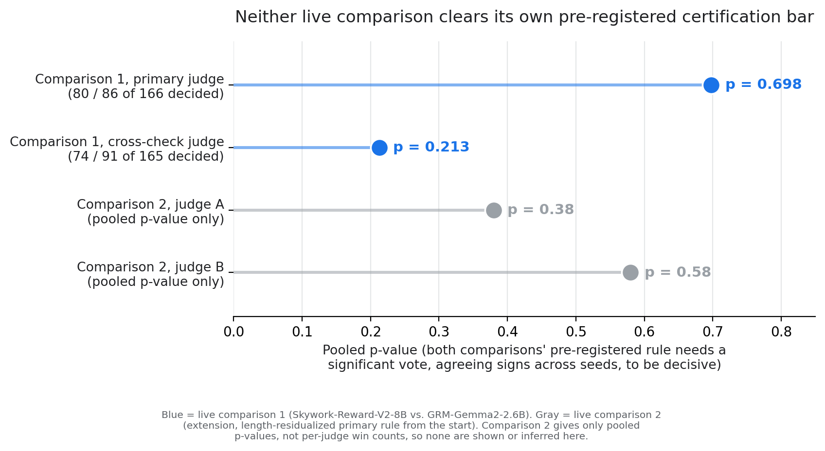
<p><img src="/assets/images/writing/reward-shopping-audit/fig5_near_tie_pvalues.png" alt="Dot plot, pooled p-value per judge for both live comparisons. None clears significance. Live comparison 1 (Skywork-Reward-V2-8B vs. GRM-Gemma2-2.6B): primary judge p = 0.698 (80 wins to 86 across 166 decided prompts), cross-check judge p = 0.213 (74 to 91 of 165 decided). Live comparison 2 (OA-DeBERTa vs. GRM-Gemma2-2.6B, length-residualized primary rule from the start): primary judge p = 0.38 (122 wins for GRM to 137 for OA-DeBERTa across 259 decided prompts), cross-check judge p = 0.58 (125 to 135 across 260 decided)." /></p>

<p>The two comparisons are not scored by the same rule, for a reason that is
chronological rather than convenient. Comparison 1 ran before the length
findings in step 4 existed and was scored under the raw vote rule in force
when it ran. Comparison 2 fixed the length-residualized rule as its primary
reading before its first training step. Each is reported under the rule that
governed it, which means comparison 1 carries a length caveat that
comparison 2’s design rules out in advance.</p>

<p>The first comparison trained a leaderboard-favored reward model,
Skywork-Reward-V2-8B, against a cheaper one it clearly outranks on a
standard leaderboard, GRM-Gemma2-2.6B, across three seeds on the 200
held-out prompts, with blind dual judging. The primary judge’s pooled vote
splits 80 wins to 86 across 166 decided prompts, p = 0.698, with a
Skywork win rate of 48.2 percent and a 95 percent interval from 40.7 to
55.7. The cross-check judge leans the same direction and is not significant
either, 74 to 91 across 165 decided prompts, p = 0.213. Its decided count
differs by one because each judge’s own noise floor sets its own ties. Both
intervals straddle 50 percent, which is the same signature as a margin
sitting below its own detection floor. One seed shows a real, individually
significant lean toward Skywork, p = 0.005 on both judges, and that lean
does not survive a length-matched re-check at any band tested. It appears
substantially explained by that seed’s variants drifting apart in response
length, the same nuisance axis step 4 shows can turn a training-time
difference into apparent reward-quality signal. The pooled verdict is a
near-tie, on a leaderboard’s top-ranked reward model against one it clearly
outranks.</p>

<blockquote>
  <p><strong>One held-out prompt from that comparison, both variants, both judges.</strong></p>

  <p><strong>Prompt</strong> (held-out set, general Q&amp;A): “What are some of the best TV shows on HBO?”</p>

  <p><strong>Skywork-trained variant’s response</strong> (336 characters): “Some highly acclaimed TV shows
produced by HBO include ‘Game of Thrones,’ ‘The Wire,’ ‘True Blood,’ ‘Westworld,’ ‘Girls,’
‘Insecure,’ ‘Ozark,’ ‘Succession,’ ‘The Leftovers,’ ‘Stranger Things,’ and ‘Big Little Lies.’
These series have garnered critical acclaim, won numerous awards, and have become cultural
phenomena in their own right.”</p>

  <p><strong>GRM-trained variant’s response</strong> (174 characters): “Some of the best TV shows on HBO
include: 1. Game of Thrones 2. The Wire 3. True Detective 4. Westworld 5. Silicon Valley 6.
Ozark 7. Veep 8. Barry 9. Watchmen 10. Succession”</p>

  <p><strong>Judge scores</strong> (each judge’s own scale, higher is better). The primary judge scores the
Skywork variant −4.69 and the GRM variant −2.70, a 1.98-point margin favoring the shorter
GRM response. The cross-check judge scores them 1.96 and 3.47, a 1.51-point margin, the
same direction. Both judges favor the shorter response on this prompt, one item among the
decided prompts the pooled p-values above are computed over.</p>
</blockquote>

<p>The second comparison trained GRM-Gemma2-2.6B against OA-DeBERTa, a reward
model already known from a companion evaluation to be substantially weaker.
It ran the same design on the extended 325-prompt pool with
length-residualized judging as its primary rule from the start. It, too,
lands as a near-tie. The primary judge splits 122 wins for GRM to 137 for
OA-DeBERTa across 259 decided prompts, p = 0.38, GRM win rate 47.1 percent,
interval 41.1 to 53.2. The cross-check judge splits 125 to 135, p = 0.58.
Both intervals straddle 50 percent. The per-seed vote signs do not even
agree in direction on either judge, and neither judge clears the
two-part rule.</p>

<p>The floor arithmetic from section 2 applies to these two comparisons as
well, with one adjustment the different statistic needs, and skipping the
adjustment would understate our own floors. Section 2’s floor is for two
independently evaluated scores. A win share is a different object. Each
decided prompt is one head-to-head trial, so the comparison is already
paired, and the compared quantity is the win-share difference D = 2w − 1,
where w is one variant’s share of the decided prompts. The variance of w is
w(1 − w)/N, the variance of D is four times that, so the standard error of
D is 2 sqrt(w(1 − w)/N) and the floor is 2.8016 times that standard error.
Comparison 1’s margin is 6 prompts out of 166 decided, 3.6 points of win
share, against a floor of 21.7 points, a ratio of 0.17. Comparison 2’s
margin is 15 of 259, 5.8 points, against a floor of 17.4, a ratio of 0.33.
The arithmetic checks against the reported tests. Converting each ratio
back to a z-score gives 0.47 and 0.93, implying p of about 0.64 and 0.35,
consistent with the measured 0.698 and 0.38, where the unpaired formula
would have implied 0.51 and 0.19, which the measured values do not support.
Both ratios say what 12 of the 15 census ratios say. The instrument that
produced these numbers could not reliably have shown a gap this size.</p>

<p>The third data point is not ours. It is AI2’s saturation caveat, quoted in
full in section 3, reached from 17 real PPO runs against real policies, the
largest downstream validation footprint of the six releases. A small,
seed-replicated, length-corrected instrument on one task and a 17-run PPO
sweep on another, built by different teams for different purposes, land on
the same reading. Once a reward model clears some basic quality bar,
further differences between good reward models are hard to detect
downstream, and a single-seed, single-horizon comparison that reports a
clean winner between two such models is more likely reporting sampling
noise than a property of the models.</p>

<p>One reading these ties do not license is a power calculation run backwards
from the observed margins, which would only restate the p-values in other
units. The sensitivity claim comes from two places fixed independently of
these results. The same instrument passes a known-null control, and it
detected an engineered half-signal reward model on 2 of 3 seeds at p values
down to 9 x 10⁻²⁹. What the instrument cannot resolve is then stated as a
floor rather than a power figure. At these decided-prompt counts, a
win-share gap under 21.7 points in the first comparison, or under 17.4 in
the second, is not reliably detectable here, and both observed margins are
far under those.</p>

<h2 id="7-what-this-method-cannot-do">7. What this method cannot do</h2>

<p>Several limits bind everything above, stated once each.</p>

<p><strong>On the comparisons that matter most, nobody knows the right answer.</strong> The
live comparisons in section 6 are writing tasks. A writing task has no
answer key, so no checker can mark a response right or wrong. When we say
one training run beat another there, the whole claim rests on two judge
models preferring its answers. We chose judges with no shared training
history with the models being judged, so that a shared blind spot would not
get counted twice, the risk Preference Leakage names (<a href="https://arxiv.org/abs/2502.01534">arXiv:2502.01534</a>).
Then we measured how independent the two judges actually are. Their scores
move together with a correlation of 0.91, and two judges that aligned
amount to about one independent opinion, not two. One more limit sits on
top of that. The length bias in step 4 was caught on a task with an answer
key, where it could be proved. The tasks here have no answer key, so we
assume the same bias operates, and that assumption is reasonable but not
provable in this setting.</p>

<p><strong>One task, one model family, one scale, few seeds.</strong> Every live comparison
runs a policy roughly 50 times smaller than a production fine-tune, at most
three seeds, for single-digit dollars. Whether a small-scale winner
predicts a production winner is untested here, the same bet the field makes
whenever a scaling law fit on small runs plans a big one. The exact
magnitudes, the sign-flip counts, the 108-to-108 tie, the seed-variance
ratios, are this project’s measurements on this setup, not universal
constants.</p>

<p><strong>The census floor assumes two independently drawn scores.</strong> Where a
paper’s two numbers share a fixed question set, the true floor runs lower,
though not by enough to close an order-of-magnitude gap. That caveat
concerns two accuracy scores on a shared question set. It does not carry
over to section 6’s win shares, which are paired head-to-head counts from
the start and take the different formula derived there. The two are
separate statistics that happen to share a multiplier, not one statistic
computed twice. Section 6’s formula carries its own assumption in exchange,
and a weaker one. It treats each decided prompt as an independent trial,
which pooling the same prompt across three seeds strains. Neither floor in
this paper is exact. Both are the right order of magnitude for the question
being asked, which is whether a margin is within reach of its instrument
at all.</p>

<h2 id="8-related-work">8. Related work</h2>

<p>This paper asks what six reward-model releases’ evaluations actually
support, how far a single-seed comparison can be trusted, and what a
cheaper discipline looks like. The table places that against the closest
neighboring work, and the paragraphs after it walk the relationships that
need more than a cell.</p>

<table>
  <thead>
    <tr>
      <th>Approach</th>
      <th>Answers</th>
      <th>Requires</th>
      <th>Our relation</th>
    </tr>
  </thead>
  <tbody>
    <tr>
      <td><strong>This work</strong></td>
      <td>What 6 releases’ evaluations support, single-seed reliability, a cheaper protocol</td>
      <td>Six papers read verbatim, a null-checked coupling pipeline, no ground-truth checker</td>
      <td>n/a</td>
    </tr>
    <tr>
      <td>Small-benchmark irreproducibility in reasoning RL (Hochlehnert et al.)</td>
      <td>Whether reported reasoning gains survive standardized re-evaluation and seed variation</td>
      <td>Released checkpoints, re-run under controlled decoding across many seeds</td>
      <td>The nearest prior statement of section 2’s argument. We compute the floor from each paper’s own stated numbers instead of re-running</td>
    </tr>
    <tr>
      <td>Static reward-benchmark-to-downstream calibration (PPE, RewardBench 2, Kim et al.)</td>
      <td>Whether a benchmark score predicts downstream RLHF/best-of-N outcomes</td>
      <td>An existing benchmark, sometimes an end-to-end calibration run</td>
      <td>Establishes the phenomenon we audit and test per-instance</td>
    </tr>
    <tr>
      <td>Underspecification mechanism account (Eisenstein et al.)</td>
      <td>Why in-distribution-agreeing reward models diverge under distribution shift</td>
      <td>Analysis of reward-model families under shift</td>
      <td>The mechanism our near-ties are consistent with</td>
    </tr>
    <tr>
      <td>Verbosity bias in LLM-as-judge (Zheng et al.)</td>
      <td>Documents that judges favor longer responses</td>
      <td>A judge model, paired responses of varying length</td>
      <td>The bias origin our judges also carry</td>
    </tr>
    <tr>
      <td>Length-Controlled AlpacaEval (Dubois et al.)</td>
      <td>Regresses length out of leaderboard win rates</td>
      <td>A leaderboard, paired length and preference data</td>
      <td>We adapt the mechanism one level up, to training</td>
    </tr>
    <tr>
      <td>Length as dominant RLHF confound (Singhal et al.)</td>
      <td>Shows length dominates reward-model training itself</td>
      <td>Analysis of reward models under RLHF</td>
      <td>Closest mechanism neighbor to nuisance-axis amplification</td>
    </tr>
    <tr>
      <td>RM length-debias engineering (ODIN, Post-hoc Calibration)</td>
      <td>Engineers a reward model less sensitive to length</td>
      <td>Access to the reward model’s training or scoring pipeline</td>
      <td>Same family, applied to the comparison check instead of RM design</td>
    </tr>
    <tr>
      <td>Known-null sanity checks (Adebayo et al., Hewitt and Liang, Sollenberger et al.)</td>
      <td>Whether a self-built evaluator is sensitive to what it claims</td>
      <td>A model, probe, or judge that can be corrupted as a null</td>
      <td>The lineage our null-check borrows directly</td>
    </tr>
    <tr>
      <td>Communication-free noise coupling (Daliri, Musco, Suresh)</td>
      <td>How to couple samples without shared communication</td>
      <td>Access to both distributions at inference time</td>
      <td>The coupling primitive we repurpose for training variants</td>
    </tr>
    <tr>
      <td>Preference Leakage</td>
      <td>How judge contamination inflates apparent preference</td>
      <td>A judge, candidates with shared or unmeasured lineage</td>
      <td>The risk our lineage-clean judge selection guards against</td>
    </tr>
  </tbody>
</table>

<p>Hochlehnert et al. (<a href="https://arxiv.org/abs/2504.07086">arXiv:2504.07086</a>) made the small-benchmark argument
first, from re-runs of released checkpoints across 20 seeds, and section 2
already states what their evidence shows and what the two-number check adds.
Ten of the fifteen census rows are AIME24 rows, so their argument covers
most of the table and the priority is theirs. Three static calibration
efforts, PPE (Frick et al., <a href="https://arxiv.org/abs/2410.14872">arXiv:2410.14872</a>), RewardBench 2 (Malik et al.,
<a href="https://arxiv.org/abs/2506.01937">arXiv:2506.01937</a>), and Kim et al. (<a href="https://arxiv.org/abs/2505.12763">arXiv:2505.12763</a>), establish that a
benchmark score does not straightforwardly predict downstream outcomes,
which is the phenomenon sections 3 and 6 audit at the practice level and
test per-instance. RewardBench 2 is also one of the six releases section 3
reads, and its volunteered saturation caveat is this paper’s independent
corroboration in section 6. Eisenstein et al. (<a href="https://arxiv.org/abs/2312.09244">arXiv:2312.09244</a>) explain
why reward models that agree in distribution can diverge once training
shifts the distribution, a mechanism our near-ties are consistent with and
do not directly test. Zheng et al. (<a href="https://arxiv.org/abs/2306.05685">arXiv:2306.05685</a>) document the
verbosity bias our judges also carry. Length-Controlled AlpacaEval (Dubois
et al., <a href="https://arxiv.org/abs/2404.04475">arXiv:2404.04475</a>) regresses length out of a static leaderboard’s
win rates unconditionally. We adapt the same mechanism one level up, to a
training-variant comparison check, and find the correction is not universally
safe, since it hurts truth-agreement in checkable settings, which their
unconditional design has no way to see. Singhal et al. (<a href="https://arxiv.org/abs/2310.03716">arXiv:2310.03716</a>)
show length dominating reward-model training itself, the closest
mechanism-level neighbor to nuisance-axis amplification, one level down
from where we find it. ODIN (Chen et al., <a href="https://arxiv.org/abs/2402.07319">arXiv:2402.07319</a>) and Post-hoc
Reward Calibration (<a href="https://arxiv.org/abs/2409.17407">arXiv:2409.17407</a>) engineer the length sensitivity out
of the reward model, the same debiasing family applied to model design
rather than to the comparison check. Adebayo et al. (<a href="https://arxiv.org/abs/1810.03292">arXiv:1810.03292</a>), Hewitt
and Liang (<a href="https://arxiv.org/abs/1909.03368">arXiv:1909.03368</a>), and Sollenberger et al. (<a href="https://arxiv.org/abs/2408.11729">arXiv:2408.11729</a>)
validate evaluators against known-null controls in vision, probing, and
code verification, and the null-check discipline here borrows that
lineage directly. Applying it a second time, to our own passing controls,
is what caught the length confound. Daliri, Musco, and Suresh
(<a href="https://arxiv.org/abs/2408.07978">arXiv:2408.07978</a>) built the communication-free noise coupling for
speculative decoding, and we repurpose it to couple two training variants.
Preference Leakage (<a href="https://arxiv.org/abs/2502.01534">arXiv:2502.01534</a>) documents the judge-contamination
risk our lineage-clean judge selection guards against, and section 7
records why that guard is partial.</p>

<p>Per-run records, evaluation outputs, cost accounting, and analysis scripts
for every measurement in this paper ship in the companion repository
released alongside it, one directory per claim, each with the command that
re-derives its headline number from the raw records. Two categories are
excluded rather than silently dropped, trained model weights and any single
record file above roughly 20 MB. Both are named with their sizes in the
directory that would otherwise hold them, and both remain available on
request.</p>]]></content><author><name>Sushant Daga</name></author><category term="paper" /><category term="reward-models" /><category term="evaluation" /><summary type="html"><![CDATA[What a benchmark's size lets it show, and why 12 of 15 recent RL papers' headline margins fall below it.]]></summary></entry><entry><title type="html">When Your Reward Model Cannot Matter: a $2 Measurement Before Training</title><link href="https://sushantdaga.com/writing/scale-tie-gate/" rel="alternate" type="text/html" title="When Your Reward Model Cannot Matter: a $2 Measurement Before Training" /><published>2026-07-28T22:00:00+00:00</published><updated>2026-07-28T22:00:00+00:00</updated><id>https://sushantdaga.com/writing/scale-tie-gate</id><content type="html" xml:base="https://sushantdaga.com/writing/scale-tie-gate/"><![CDATA[<p>You are picking between two ways of grading a model’s attempts during training. One is a
checker: it reads an answer and says right or wrong, nothing in between (the rule-based setup
known as RLVR, reinforcement learning with verifiable rewards). The other is a reward model: a
trained scorer that reads the same answer and hands back a number, a graded sense of how good
the attempt was, even among the ones that are technically wrong. Think of two graders marking the
same stack of papers. One carries a stamp, PASS or FAIL. The other writes a score out of a
hundred. Hand both of them two failing answers, one nearly right and one hopeless: the stamp
reads FAIL on each, the score reads a 40 on one and a 5 on the other. You run a cheap comparison
between a checker and a reward model at small scale and one wins. Will that winner still win once
you train at the size you actually ship?</p>

<p>The closest evidence is from pretraining optimizer comparisons (<a href="https://arxiv.org/abs/2512.05620">arXiv:2512.05620</a>). Even careful,
scale-aware studies there disagree with each other, from a steady 2x speed advantage at one end to
nothing at the other, over the same range of model sizes. This piece brings a cheap quantity to
that bet, the fraction of training questions where the training update is mathematically forced to
be exactly zero, and traces it across two tasks and two model sizes before any training starts.
The quantity itself is not new. DAPO (<a href="https://arxiv.org/abs/2503.14476">arXiv:2503.14476</a>) named the zero-advantage group in 2025 and
built a remedy around it, dynamic sampling, which keeps drawing until a batch carries enough groups
whose attempts disagree. What this piece adds is the measured trace: the same rate read on the same
task at two model sizes, treated as something to forecast from rather than something to filter
away.</p>

<h2 id="what-this-piece-found">What this piece found</h2>

<ul>
  <li>The training method in question (GRPO-family reinforcement learning) learns
only from disagreement among its own sampled attempts. When every attempt at a
question gets the same grade, the weight update for that question is exactly
zero, proven for the GRPO family (<a href="https://arxiv.org/abs/2607.00152">arXiv:2607.00152</a>), which states the result
for the on-policy first step, and approximately zero in the common setups that
add a KL penalty.
Call the fraction of questions where all attempts tie the shut-gate rate.
Reward choice can only matter where the gate is open.</li>
  <li>The gate moves with difficulty and with model size, measured before any
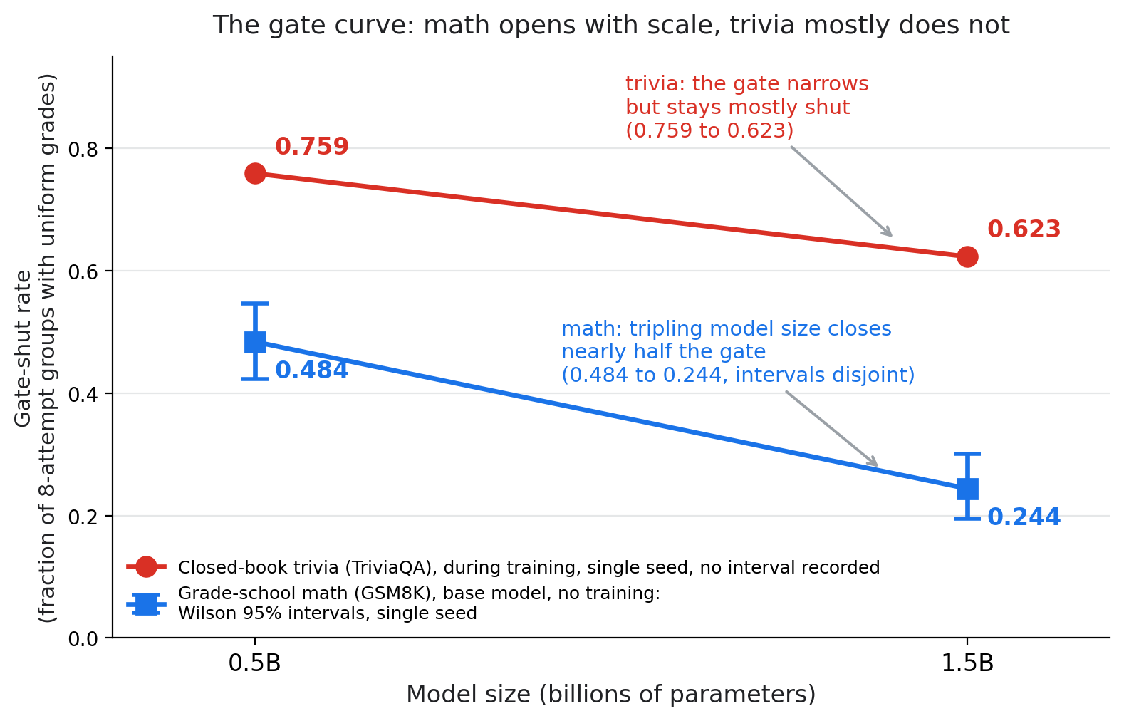
training: a harder task left the gate shut about 3x as often on the same model,
and tripling model size (Qwen2.5-0.5B to 1.5B) roughly halved the shut-gate
rate on grade-school math, 0.484 to 0.244. Single-seed readings.</li>
  <li>Where the gate was mostly open, 3 trained reward-model variants landed 1.6 to
5.4 points above the plain right/wrong checker, every one of those gaps inside
the roughly 6-point margin a single training run cannot resolve. A consistent
direction, not a proven ranking. Single-seed.</li>
  <li>What the study’s own rule ends up calling: no winner. Three runs differing only in random seed
compared the reward model GRM-Gemma2-2.6B (published as
Ray2333/GRM-Gemma2-2B-rewardmodel-ft, named for its 2B-class Gemma-2 base,
which carries 2.6 billion parameters) against a copy of itself trained with
half its reward signal replaced by random noise, on the instruction-following
task, scored by the FsfairX judge on length-corrected votes. Two seeds favored
the intact signal by wide margins (131 wins to 87 and 145 to 68). One leaned
the other way (83 wins to 108 of 191 decided votes, meaning votes where the
judge saw a difference, and a fair coin would produce a split at least this
uneven about 8% of the time, p = 0.082). This piece’s bar for declaring a
winner asks two things at once: a pooled per-prompt majority vote significant
on an exact two-sided binomial test, and every seed’s own sign agreeing with
the majority. In plain terms, each question gets one combined verdict from the
three runs, that tally has to be strong enough that chance explains it poorly,
and no individual run may point the other way. The combined verdict here does
favor the intact signal, 147 questions to 104 with 74 undecided, p = 0.0079.
The dissenting seed points the other way, so the rule calls no winner. What
it does support is a bound taken from that seed,
picked because it is the seed that failed rather than because it is
representative: on that seed the intact signal’s win share sits between 36%
and 51% at 95% confidence, anywhere from clearly behind to dead even, never
ahead. The other 2 seeds each bound the same quantity entirely above 50%.
Quoting the worst of the three is the conservative choice, not a reading of a
typical run.</li>
  <li>One before-you-train forecast has been scored against real trained outcomes, in
three settings. On closed-book trivia the plain checker finished 2.2 points
ahead, an interval of [0.2, 4.4] at 95% confidence that excludes zero, and about
9% of that gap survived once answers were credited for content rather than exact
wording. On the two grade-school-math settings the intervals span zero at both
evaluation pool sizes tried. The zero-update mechanism is arithmetic. The tie
counts are measurements that repeat. Three settings decide nothing on their own.</li>
  <li>Settling it costs $20 to $60 at the scale this piece works at, and about $95 to
$280 at the 7B-class scale a skeptical reader should demand.</li>
</ul>

<h2 id="1-the-gate-why-reward-choice-sometimes-cannot-matter">1. The gate: why reward choice sometimes cannot matter</h2>

<p>GRPO (group relative policy optimization), the training recipe behind this comparison, samples
several attempts at the same question, grades each one, and nudges the model toward whichever
attempts scored better than the others in that group. It is a relative judgment, not a fixed bar:
like a grade set by where you land relative to the rest of the room, not by a fixed cutoff. Score
70 on an exam everyone aced and you are below average. Score the same 70 where everyone struggled
and you are top of the class. The exam did not change. Your standing relative to the group did.</p>

<p>Push that to its edge. Ask the model the same question 8 times and every attempt comes back
wrong, or every attempt comes back right. Nobody stood out, because everybody matched. DAPO
(<a href="https://arxiv.org/abs/2503.14476">arXiv:2503.14476</a>) named this in 2025, informally, calling it the gradient-decreasing problem and
making it the motivation for its dynamic sampling filter. A 2026 paper derived it as near-zero
advantage collapse (<a href="https://arxiv.org/abs/2605.21125">arXiv:2605.21125</a>, submitted 20 May 2026), and a proof about six weeks after
that (<a href="https://arxiv.org/abs/2607.00152">arXiv:2607.00152</a>, submitted 30 June 2026) makes it exact. When a group is uniform like that,
the update to the model from that group is not small. It is precisely zero. Whatever the training
signal is, a plain checker or an elaborate learned scorer, it never gets a vote, because there was
no disagreement within the group for it to break.</p>

<p>That exactness carries one condition worth stating in plain sight. The proof is stated for the
on-policy first step of the group-relative objective, and its own limitations section sets
clipping, the KL penalty to a reference policy, off-policy staleness, and non-binary rewards aside.
Common implementations do carry a KL term or an entropy bonus, and those terms do not vanish on a
tied group, so in a real training loop the honest word is approximately zero rather than exactly
zero.
The part that stays exactly zero is the part this piece is about: the reward’s own contribution.
A regularizer pulls the model toward a reference policy whatever the grades were, which is another
way of saying reward choice still gets no vote there.</p>

<p>Call this a gate. A shut gate carries no training signal no matter which reward graded it. An
open gate, where attempts actually disagree, is the only place reward choice can act.</p>

<p>Two real questions from a base-model GSM8K measurement show both cases.</p>

<table>
  <thead>
    <tr>
      <th>Case</th>
      <th>Question (abridged)</th>
      <th>Gold answer</th>
      <th>8 sampled attempts</th>
      <th>Outcome</th>
    </tr>
  </thead>
  <tbody>
    <tr>
      <td>Gate shut</td>
      <td>“A factory used to make tractors, but now makes silos… What percentage more are they making per day now?”</td>
      <td>10</td>
      <td>120, 14.14, 100, 122, 24, 34, 20, 9.9</td>
      <td>None of the 8 attempts match the gold answer. Nobody stood out, gate shut.</td>
    </tr>
    <tr>
      <td>Gate open</td>
      <td>“Comet Halley orbits the sun every 75 years… How old was Bill when he saw the Comet for the first time?”</td>
      <td>15</td>
      <td>15, 2, 45, 60, 0, 90, 32.17, 60</td>
      <td>One attempt matches. It disagrees with the other 7, so this group has something for reward choice to act on.</td>
    </tr>
  </tbody>
</table>

<p>How often the gate is open is arithmetic, not a discovery. If a model answers a question correctly
with probability <em>p</em>, and you sample <em>n</em> attempts, the chance every attempt lands the same way is</p>

<div class="language-plaintext highlighter-rouge"><div class="highlight"><pre class="highlight"><code>P(all n agree) = p^n + (1-p)^n
</code></pre></div></div>

<p>The first term is the chance all n attempts land right, the second the chance all n land
wrong, and a tie is either one.</p>

<p>At p = 0.9 and n = 8: 0.9^8 + 0.1^8 = 0.430. A question the model has nearly mastered still ties
43% of the time. Put p = 0.1 into the same formula and it returns the same 0.430. Put p = 0.5 in
and it bottoms out at 0.008. The curve is U-shaped in p, high at both ends and lowest where the
model is right about half the time.</p>

<p>Which way capability moves the gate therefore depends on which side of that minimum a question
sits. Climbing from p = 0.1 toward p = 0.5 drives the tie rate down. Climbing from p = 0.5 toward
p = 0.9 drives it back up. The questions measured here sit overwhelmingly on the low side, and the
composition of their ties says so directly. On base-model GSM8K at 0.5B, all 121 tied questions
out of 250 were tied all-wrong and not one was tied all-right, and at 1.5B the tied mass splits
into 19.2% tied all-wrong and 5.2% tied all-right. That is why the table below shows the gate
opening as models get bigger, while the same arithmetic says material a model has mostly mastered
shuts it again, for the same reason a coin that lands heads 95% of the time gives you 8 heads in a
row far more often than a fair coin does. Both readings are the one curve, seen from its two
sides.</p>

<p>That the gate moves with capability is expected by construction. Which direction it moves is not,
because that is set by where a task’s questions sit against the minimum, and that is a measurement
rather than a deduction. Whether the gate is the specific channel through which capability changes
training outcomes, rather than merely correlated with them, is the open, unproven claim this piece
is actually built on.</p>

<p>Measured shut-gate rates, before and during training, across tasks and sizes:</p>

<table>
  <thead>
    <tr>
      <th>Task</th>
      <th>Model size</th>
      <th>Shut-gate rate</th>
      <th>Reading</th>
    </tr>
  </thead>
  <tbody>
    <tr>
      <td>Harder math (MATH, Level 3-5), trained</td>
      <td>1.5B</td>
      <td>0.62-0.64</td>
      <td>harder task, trained: mostly shut</td>
    </tr>
    <tr>
      <td>Grade-school math (GSM8K), trained</td>
      <td>1.5B</td>
      <td>~0.206</td>
      <td>same model, easier task: mostly open</td>
    </tr>
    <tr>
      <td>Closed-book trivia (TriviaQA), in training</td>
      <td>0.5B</td>
      <td>0.759</td>
      <td>recall task: mostly shut</td>
    </tr>
    <tr>
      <td>Closed-book trivia (TriviaQA), in training</td>
      <td>1.5B</td>
      <td>0.623</td>
      <td>same task, tripled size: narrows, still mostly shut</td>
    </tr>
    <tr>
      <td>GSM8K, base model, no training</td>
      <td>0.5B</td>
      <td>0.484 [0.423, 0.546]</td>
      <td>untrained: about half of groups already tie</td>
    </tr>
    <tr>
      <td>GSM8K, base model, no training</td>
      <td>1.5B</td>
      <td>0.244 [0.195, 0.301]</td>
      <td>tripling size: gate drops by nearly half, intervals disjoint</td>
    </tr>
  </tbody>
</table>

<p><em>Bracketed numbers are 95% confidence intervals, the plausible range for the true value, not the
measurement itself. All rows single-seed. The 2 trivia rows are in-training rates from the earlier
TriviaQA runs described in section 5, read at sampling temperature 1.2 against 0.8 for every other
row and over a different training horizon, so they belong in the table as separate readings and not
as numbers to subtract from the base-model rows beneath them. The 2 trained rows are also not the
same kind of reading. The grade-school-math rate is what the checker saw live in its own run. The
harder-math rate is a right/wrong rate recomputed afterwards from the stored attempts, which is
what a checker would have seen on that task. The runs graded by a reward model there almost never
produced an exact tie in their own continuous scores, so their live rate sat near zero.</em></p>

<p><img src="/assets/images/writing/scale-tie-gate/fig2_gate_curve.png" alt="Line chart of the shut-gate rate against model size, 0.5B versus 1.5B. The GSM8K line, a base-model reading taken before any training and drawn with 95% intervals, drops from 0.484 to 0.244. The TriviaQA line, an in-training reading from the earlier runs and carrying no recorded interval, stays high and narrows only slightly, 0.759 to 0.623." /></p>

<p><strong>The shut-gate rate falls with scale on both tasks measured here, but starts and ends much higher
on the recall task than on the reasoning task. The 2 lines are not one measurement. The math line
is a base-model reading and the recall line is an in-training reading from the earlier runs, so
read each line’s own slope and not the vertical distance between them.</strong></p>

<p>Task difficulty moves the gate by a factor of 3 on one fixed-size model (MATH’s 0.62-0.64 against
GSM8K’s 0.206). Model size moves it by roughly half on one fixed task (0.484 to 0.244). The two
trivia rows show a different regime. Tripling model size narrows the gate from 0.759 to 0.623 but
leaves it mostly shut, because what blocks a recall question is a missing fact, not shaky
execution, and a bigger model knows more facts while still missing most of the rare ones. In the
terms of the U-shaped curve, recall questions sit further out on the low side than math questions
do, so the same climb in capability buys less gate. Section 5 returns to why that distinction
matters.</p>

<p>One scope limit belongs here. The zero-update proof covers GRPO-family, group-relative methods.
An older style of reinforcement learning, PPO (proximal policy optimization) with a learned value
function as its baseline (Schulman et al. 2017, <a href="https://arxiv.org/abs/1707.06347">arXiv:1707.06347</a>), scores each attempt against
that separately learned baseline instead of against its own siblings in a group. Because PPO’s
advantage is attempt minus a learned function’s estimate, not attempt minus the group’s own mean,
a uniform group does not automatically zero it out the way group-normalization does. Whether an
analogous gate exists there anyway has not been proven or measured. It is an open corner of the
theory, not a claim this piece makes about PPO.</p>

<h2 id="2-the-155-reading-measure-the-gate-before-you-train">2. The $1.55 reading: measure the gate before you train</h2>

<p>The gate is cheap to read. Sample a batch of rollouts from the model you plan to train, at the
size and on the task you actually care about, grade them with your checker, and count how many
groups came back uniform. No training involved, pure inference. The base-model gate curve above
cost about $1.55 in total cloud compute, most of it a single small AWS
instance running for under two hours.</p>

<p>Reading the gate also explains a piece of training machinery worth naming precisely, because it
is easy to confuse with an unrelated setting of the same name. One of the reward variants tested
on GSM8K is a tie-break blend: reward = checker grade + epsilon x within-class reward-model rank,
where epsilon = 0.1. This epsilon is not GRPO’s clipping epsilon from the policy-gradient
objective. It is a blend weight. It adds a ranked nudge inside each same-grade class of a group,
which in a group the checker already called a tie means the whole group at once, and in a mixed
group means the right attempts ranked among themselves and the wrong ones among themselves, using
GRM-Gemma2-2.6B’s own ranking to do the ranking. Because an attempt graded right scores at least
1.0 and an attempt graded wrong scores at most 0.1, the blend can never overrule the checker’s
ordering in a group where attempts actually disagree. On the GSM8K run, the tied groups where the
blend is the entire signal made up about 21% of scored attempts (the tie-break blend’s own
shut-gate rate was 24% against the checker-only variant’s 20.6%): that is the slice where epsilon
decides everything rather than nothing. One caveat worth carrying: after GRPO’s own per-group
advantage normalization, whatever non-zero signal epsilon contributes inside a formerly tied group
gets rescaled to the group’s full standardized strength, not held down at its nominal 0.1 weight.
It acts small in the reward, full strength in the update.</p>

<p>On that same GSM8K run, where the gate was mostly open, three trained reward-model variants all
beat the plain right/wrong checker (the binary verifier in GRPO-style training, RLVR):
GRM-Gemma2-2.6B by 5.4 points, the epsilon = 0.1 tie-break blend by 4.2 points,
Skywork-Reward-V2-Qwen3-8B by 1.6 points.</p>

<table>
  <thead>
    <tr>
      <th>Variant</th>
      <th>Gap over the checker</th>
    </tr>
  </thead>
  <tbody>
    <tr>
      <td>GRM-Gemma2-2.6B</td>
      <td>+5.4 points</td>
    </tr>
    <tr>
      <td>Epsilon = 0.1 tie-break blend</td>
      <td>+4.2 points</td>
    </tr>
    <tr>
      <td>Skywork-Reward-V2-Qwen3-8B</td>
      <td>+1.6 points</td>
    </tr>
  </tbody>
</table>

<p>The middle row needs a caution the other two do not. The blend’s epsilon cancels under GRPO’s own
per-group standardization, worked through at the end of this section, so whatever produced that
run’s 4.2-point margin, it was not the amount of blend weight the variant is defined by. That row
is a recorded outcome with its mechanism unaccounted for.</p>

<p>Part of that edge is mechanical rather than a reward-quality difference: the loss normalizes over
the full batch of sampled sequences, live and dead groups alike, so the checker’s own dead groups
(20.6% of the batch) contribute zero to the numerator while still counting in the denominator,
diluting its per-step gradient by roughly 21%. Even accounting for that, every gap sits inside the
roughly 6-point margin one single-seed run cannot rule out (worked out in section 4), so this is a
directional pattern, not a proven one. A second signal comes from a related follow-up run: raising the
tie-break blend’s own weight from epsilon = 0.1 to epsilon = 0.2, doubling how much
GRM-Gemma2-2.6B’s ranking counts inside tied groups, moved mean accuracy over the last 3 checkpoints
from 55.9% down to 53.3%, a 2.6-point move. That move is single-seed and sits inside the same
roughly 6-point margin one run cannot rule out. Its direction, more weight on the reward model’s
ranking producing a worse score, does not support the story that the reward model ranks better
than the checker.</p>

<p>Those last two paragraphs are in tension. The normalization caveat says the standardized update
inside a formerly tied group does not depend on epsilon’s size, because doubling the spread also
doubles the divisor the group is standardized by. So doubling epsilon changes nothing at all in
exactly the groups the blend was designed for. The only place it can act is inside groups that
already mix right and wrong attempts, where it shifts how much the within-class ranking counts
against the grade itself. The 2.6-point move is therefore not a dose-response reading of the
tie-break mechanism, and single-seed run-to-run variation stays the plainest available explanation
for it.</p>

<h2 id="3-the-forecast-scored-three-settings-none-of-them-decisive">3. The forecast, scored: three settings, none of them decisive</h2>

<p>Everything above measures a mechanism. It does not, on its own, show that mechanism predicts
training outcomes. That requires a forecast locked in before training, then checked against what
actually happened. This piece has one real attempt at that: run once, single-seed, and built to
map the terrain rather than to settle it, a gate-and-composition reading taken on a base
model, a prediction written down from it, then a real GRPO comparison between the plain
right/wrong checker (the binary verifier in GRPO-style training, RLVR) and a reward model,
GRM-Gemma2-2.6B, trained to convergence and scored against that prediction.</p>

<p>One of the three settings turns entirely on how an answer is scored, so it goes first. On
closed-book TriviaQA at 0.5B, in the gate-validation run, which is a different experiment from the
earlier TriviaQA runs section 5 describes, the checker finished 2.2 points ahead, [0.2, 4.4]. That
interval excludes zero, so on the strict scoring the two variants came apart, against a prediction
of a tie. Both had learned, 8.7 to 10.9 points over their own untrained baseline. Then a looser
scoring, written into the plan before the run and triggered by this exact outcome, was applied: an
answer counts if its content is right even when its exact string is not. About 9% of the 2.2-point
gap survived it, leaving 0.2 points. The reward-model variant’s answers had also drifted 1.7 tokens
terser over training, exactly the kind of change a strict string-match checker reads as a teaching
difference. Both facts point the same way, that most of the gap is the reward model reshaping the
form of its answers rather than teaching the model less, and that reading comes from one
single-seed run rather than a settled mechanism. Which of the two scorings you apply decides
whether this setting separated or tied.</p>

<p>The other two settings are the actual test of the theory. One convention governs every gap and
interval in this section: each is written as checker minus reward model, so a positive number means
the checker ahead and a negative one means the reward model ahead. On GSM8K at 0.5B, where a tie
was predicted, the gap came in at +1.0 point, [-3.8, +5.6], both variants gaining 21 to 22 points
over base and converging at the same training step. On GSM8K at 1.5B, where the prediction was a
moderate reward-model edge of about -2 points, the gap also came in at +1.0 point, [-3.2, +5.2],
with the two runs stopping at different step counts (175 and 100). A later re-check on 2,000
questions instead of 500 narrowed both intervals roughly in half (9.4 points wide to 4.8, 8.4 to
4.5), the larger question pool buying more precision on the same two comparisons. The 0.5B pair now
reads +2.35 points, [-0.05, +4.75], a lower bound sitting 0.05 points from crossing zero. The 1.5B
pair now reads -0.65 points, which is the reward model ahead by that much, [-2.9, +1.6].</p>

<p>What the two GSM8K rows agree on, independent of how any single verdict is scored, is the size of
what is at stake: reward choice moved final accuracy by about a single point either way, well
inside noise, while the checker and GRM-Gemma2-2.6B each taught the
model 19 to 22 points wherever the gate was open enough to let training happen at all. The whole
validation, including the recall-task attempt, cost about $12 of cloud compute, cheaper than a
single seed of the train-it-twice bet this piece opened with.</p>

<table>
  <thead>
    <tr>
      <th>Task / size</th>
      <th>Predicted</th>
      <th>Measured gap</th>
      <th>Interval</th>
    </tr>
  </thead>
  <tbody>
    <tr>
      <td>TriviaQA, 0.5B</td>
      <td>Tie</td>
      <td>+2.2 points strict, +0.2 points content-tolerant</td>
      <td>[+0.2, +4.4] (strict scoring, n=500)</td>
    </tr>
    <tr>
      <td>GSM8K, 0.5B</td>
      <td>Tie</td>
      <td>+1.0 point (n=500), +2.35 points (n=2,000)</td>
      <td>[-3.8, +5.6] (n=500), [-0.05, +4.75] (n=2,000)</td>
    </tr>
    <tr>
      <td>GSM8K, 1.5B</td>
      <td>Moderate reward-model edge (about -2 points)</td>
      <td>+1.0 point (n=500), -0.65 point (n=2,000)</td>
      <td>[-3.2, +5.2] (n=500), [-2.9, +1.6] (n=2,000)</td>
    </tr>
  </tbody>
</table>

<p><em>Measured gaps and intervals are checker minus reward model: positive means the checker ahead,
negative means the reward model ahead. The trivia interval belongs to the strict scoring. The
content-tolerant pass is a re-score of the same answers, not a second interval.</em></p>

<p>Read across the three, the forecasts landed like this. The tie predicted on grade-school math at
0.5B held at 500 questions and, at 2,000, moved to a checker lean of 2.35 points whose lower bound
stops 0.05 points short of zero: still spanning zero, and only just. The reward-model edge predicted
at 1.5B is not established at either pool size, and the point estimate did cross to the predicted
side at 2,000 questions, where the interval contains both zero and the predicted 2-point edge. The
tie predicted on trivia is the one contradicted at face value, by a gap whose interval excludes
zero, and also the one whose contradiction turns on a scoring choice. Both math settings moved when
the pool grew rather than settling.</p>

<p>One asymmetry in the scoring belongs on the record. The content-tolerant re-score was run only on
the trivia setting, where answers are free text and a truncated string is marked wrong for its
form. The math settings are graded on the final number, which already counts an answer wherever in
the response it appears and in whatever notation, so the same loosening has no counterpart there
and none was run.</p>

<p>The gate reading has been through one scored test so far, in three settings, and no setting came
back decisive. Two of them cannot separate the predicted effect from no effect at the precision
they were run at. The third turns on which of two defensible scorings is applied. That is not
enough to lean on. It is enough to keep going, and section 6 works out what settling the question
would cost at two scales.</p>

<h3 id="one-prediction-offered-and-untested">One prediction, offered and untested</h3>

<p>A continuous reward mostly does not have this gate, which offers one further, untested
consequence. Re-scoring already-stored math-style rollouts with a trained reward model
(Skywork-Reward-V2-Qwen3-0.6B) instead of the checker collapsed the shut-gate rate from 22.3-57.2%
under the checker to under 1% under the reward model, on the same stored sequences, because a
continuous number rarely lands on exactly the same value twice, where a binary label folds many
different wrong answers into the same 0. If the gate is really the channel scale acts through,
tasks graded by a continuous judge instead of a checker, where the gate is already mostly open,
should show little to no crossover as you scale up: a richer signal should look however good or
bad it looks at the smallest scale you can afford and stay close to that. This is offered as a
falsifiable consequence of the gate story, not a second finding: it has not been tested against
any trained outcome.</p>

<h2 id="4-seed-noise-measured-and-what-it-costs-to-beat">4. Seed noise, measured, and what it costs to beat</h2>

<p>Two things are set at random before a training run starts: where the weights begin and the order
the data arrives. Change the seed and the final model differs, everything else held fixed.</p>

<p>A separate experiment in this program measures exactly how much that matters. Same Qwen2.5-1.5B
model, same GRPO recipe, on the Dolly instruction-following dataset: 3 independently seeded runs
each trained one policy against GRM-Gemma2-2.6B’s full reward signal and a matched twin against the
same reward model with half its signal replaced by random noise every step. The three runs differ
only in seed. Two judge models, fsfairx and mistral, then scored both final policies head-to-head
on one fixed set of 325 held-out questions, drawn once and put in front of every seed unchanged.</p>

<p>Two different numbers can come out of the same seed, and it matters which one you read. Tallies
are the raw win, loss, and tie counts a judge casts. Scores are the judge’s own continuous number
for each attempt, and a length-residualized score corrects that number for something correlated
with it, here answer length, before counting a win. The correction is a simple regression: fit</p>

<div class="language-plaintext highlighter-rouge"><div class="highlight"><pre class="highlight"><code>score_diff = beta0 + beta1 x length_diff
</code></pre></div></div>

<p>across every scored pair, then judge each pair on its residual (its score difference with the
length-predicted component removed) rather than its raw score difference. Fit on this program’s
own data (fsfairx judge), beta1 = 0.0035 with R-squared = 0.37, meaning every extra token of
length predicts 0.0035 more raw score-difference, and length differences explain 37% of the
variance in raw score differences. Worked example: two attempts differ by 0.05 in raw score, and
the reward-model-scored one also ran 20 tokens longer. Length alone predicts 20 x 0.0035 = 0.070
of that gap, more than the whole observed difference, so the residual is 0.05 - 0.070 = -0.020:
once you remove what length alone would predict, this attempt actually looks worse, not better.
That is why the same seed can flip sign between the two analyses.</p>

<table>
  <thead>
    <tr>
      <th>Seed</th>
      <th>Raw tally (GRM wins-losses-ties)</th>
      <th>Residualized tally (wins-losses-ties)</th>
      <th>Residualized p</th>
    </tr>
  </thead>
  <tbody>
    <tr>
      <td>1</td>
      <td>185-57-83</td>
      <td>131-87-107</td>
      <td>0.0035</td>
    </tr>
    <tr>
      <td>2</td>
      <td>106-109-110</td>
      <td>83-108-134</td>
      <td>0.082</td>
    </tr>
    <tr>
      <td>3</td>
      <td>202-41-82</td>
      <td>145-68-112</td>
      <td>&lt;0.001</td>
    </tr>
  </tbody>
</table>

<p><em>p is an exact two-sided binomial test on the decided (non-tied) votes per seed, the pre-registered
primary analysis (fsfairx judge).</em></p>

<p>The two-part rule this piece holds itself to is the one stated at the top, and both halves of it do work
here. Across the same 325 questions, pool the three seeds question by question, take the majority
verdict on each one, and test that tally: 147 questions favor the intact signal against 104 for the
noise-injected twin, with 74 undecided, a split at least this uneven being one a fair coin produces
about 8 times in a thousand (p = 0.0079). That clears the significance half on its own. The second
half asks every seed’s own direction to agree with the majority, and seed 2’s does not. The rule calls no winner, and the pooled number is exactly
what the second half exists to stop anyone reporting by itself.</p>

<p>On the raw tally, seed 2 reads as a near-exact coin flip, 106 to 109. On the residualized reading,
that same seed leans the other way, 83 to 108, favoring the noise-injected twin. The measurement
carries its own imprecision, and the size of it is knowable. Each seed’s tally is one judged pass
over the same 325 questions and inherits that pool’s sampling error, and seed 2’s lean sits inside
that error rather than outside it, which is what its p = 0.082 says. What the sampling error does
not cover is the distance between that seed and the other two, which land on the opposite side at
p = 0.0035 and p &lt; 0.001. Three runs that differ only in seed came apart further than the
instrument reading them wobbles.</p>

<p>This can be costed the way an engineer costs a manufacturing tolerance. A $0 re-analysis of this
data split the uncertainty in a pooled 3-seed verdict into 3 pieces: how much comes from
which seed you drew, how much from how many test questions you checked against, how much from
disagreement between judges. At this one measured scale, the seed piece is about 12.4 times larger
than the test-question piece and roughly 1.1 million times larger than the judge-disagreement
piece, and the current 3-seed pooled margin of error sits at 7.25 percentage points. Spending the
next $5 on a fourth seed plus a few hundred more test questions cuts that margin to about 6.2
points. Spending the same $5 entirely on test questions barely moves it, to about 7.1 points,
because test-question noise was never where the disagreement was coming from. One boundary on
this advice: it concerns the plain pooled margin, the width of the combined verdict, and nothing
else. The two-part rule puts the sign condition on top of that margin, and
under both conditions at once the arithmetic changes. Each added seed sharpens the pooled test
and at the same time makes agreement in direction harder, because a new seed is one more chance
to point the other way and its own precision is set by the question pool rather than by how many
seeds there are. The two effects mostly cancel, so seeds stop paying after the third, while
growing the question pool shrinks every seed’s own noise directly and keeps paying. The fuller
cost accounting, including the per-dollar ranking across seeds, test questions, and judges, is worked out
in a companion piece published alongside this one, <a href="/writing/same-dice-different-winners/">“Same RL Recipe, Different Seed, Different
Verdict: Here’s a Training Comparison You Can Trust.”</a> This section keeps only the ratio the gate
story needs.</p>

<p>One number here is a measurement, and one is a design constant, and they should not be confused
with each other. The 6-point margin used in section 2 is not measured seed variance. It is
standard power arithmetic, computed and locked in before training started: at n = 500 held-out
questions and roughly 50% base accuracy, the standard error on the difference between two
variants is</p>

<div class="language-plaintext highlighter-rouge"><div class="highlight"><pre class="highlight"><code>SE = sqrt(2 x 0.5 x 0.5 / 500) ≈ 0.03 (about 3 percentage points)
</code></pre></div></div>

<p>and 2 standard errors of headroom, the usual bar for calling a gap real rather than noise, is
about 6 points. The 7.25-point figure above is a different, measured quantity: the actual pooled
margin of error this program’s own 3-seed Dolly runs achieved, on a different task, at a different
point in training.</p>

<p>Connect this back to the optimizer comparison the piece opened with, where scale-aware studies of
the same optimizers land anywhere from a steady 2x speed advantage down to none at all
(<a href="https://arxiv.org/abs/2512.05620">arXiv:2512.05620</a>). Nothing measured here settles that literature. What it offers is a cheaper
candidate explanation to rule out first: if a comparison run at a single seed there carries
anything like the seed spread measured in this section, disagreement of that shape can arise with no
scale-transfer effect at all. Whether the seed-noise term itself
shrinks, holds steady, or grows as models get bigger has not yet been measured. That is exactly the
next experiment section 6 puts a cost on.</p>

<p><img src="/assets/images/writing/scale-tie-gate/fig3_seed_noise.png" alt="Two log-scale bar charts. Left: contribution to a training comparison's verdict variance, seed 1.46e-02, test questions 1.18e-03, judge 1.30e-08. Right: variance-reduction per dollar spent, seed 3.76e-04 (1st), test questions 7.32e-05 (2nd, about 5x worse), judge 6.10e-10 (3rd, about 613,000x worse)." /></p>

<p><strong>One more seed beats more test questions beats more judges, by orders of magnitude, at the one
scale this has been measured.</strong></p>

<h2 id="5-ignorance-or-unreliability-two-reasons-a-gate-stays-shut">5. Ignorance or unreliability: two reasons a gate stays shut</h2>

<p>A shut gate on a recall question and a shut gate on a math question can look identical in the
count and mean something different underneath. Answering “who is the Norse god of thunder” is
closer to a light switch than a dial: either the fact sits in the model’s weights and comes out,
or it does not, and no amount of resampling finds it. A shut gate here, all 8 attempts landing the
same way, is mostly a tie of ignorance. Getting a multi-step math problem right depends on which
path the model takes, where a digit gets dropped, which step goes sideways: the same underlying
competence can land right on one attempt and wrong on the next. A shut gate here is more often a
tie of unreliability, the correct chain reachable but not landed on consistently, which is exactly
the kind of gap reinforcement learning is built to close.</p>

<p><img src="/assets/images/writing/scale-tie-gate/fig4_tie_composition.png" alt="A tied group (all eight attempts land the same way) branches into two cases. Left, tie of ignorance: closed-book trivia, the fact isn't in the model's weights, resampling never finds it, training can't convert this tie. Right, tie of unreliability: grade-school and harder math, the correct chain is reachable but not landed on every time, training can close this gap." /></p>

<p><strong>A shut gate’s size tells you how much of a batch could carry a signal. Its composition tells you
whether that signal, once carried, has anything to teach the model.</strong></p>

<p>This program’s own numbers back the split, and they cut both ways. Two different TriviaQA
experiments sit behind what follows, and they say different things. The earlier pair of runs (0.5B
and 1.5B, sampling temperature 1.2, 175 training steps) held at its base rate across every measured
checkpoint under all three
rewards, including the plain right/wrong checker (the binary verifier in GRPO-style training,
RLVR). That pair carried no measured baseline at step 0 and its first checkpoint already sat at
base rate, which leaves its gate measurement as the part worth leaning on and its accuracy
trajectory as the part that cannot decide anything: “no learning” cannot be cleanly separated there
from “a small early bump then flat.” The later gate-validation run is a different experiment, at 0.5B only, stopped at 100 steps,
and in it both variants did learn: the checker by 10.85 points over its own untrained baseline
[8.2, 13.7] and the reward model by 8.65 points [6.1, 11.3]. Both sampled at the same temperature,
1.2. What differs is the training horizon (175 steps against 100), the model sizes covered (both
against 0.5B alone), the setup each ran on, and the baseline each was measured against, since only
the later run measured its own untrained starting point and its own base-model tie count. They are
separate experiments rather than two readings of one, and no gap between them is worth computing.</p>

<p>That means the ignorance reading rests on composition rather than on any learning null. In the
later run’s own base-model count of the exact questions it went on to train against, the trivia
gate read 0.7700 [0.7311, 0.8047], and every tied question in it was tied all-wrong, with zero
questions tied all-right. Pure fact-ignorance ties, no mastery ties at all, which is the signature
the split predicts for a recall task and is evidence in a way that a flat training curve is not.</p>

<p>On the harder math task the count reads 61.7% all-wrong, and it needs its scope attached to be read
at all. It is a share of sampled groups rather than of questions: four training variants each made
a single pass over the same 480 questions, and the 61.7% pools all 1,920 of those groups. The
training runs beside it cannot carry an ignorance reading on their own. No variant there separated
from its own untrained accuracy of 0.203. The four finished between 0.190 and 0.211, and at 384
evaluation questions one standard error is 2.05 points, so every one of those gaps sits inside a
single standard error. That configuration also ran 60 steps on a reduced budget, and the fuller
configuration the task was originally scoped for was never run. This task is
therefore in the same position as the earlier trivia pair: “no learning” and “too little training
to tell” cannot be separated here, and what the run contributes is its count of ties, not a verdict
on what reward choice did.</p>

<p>On grade-school math the comparable count is a base-model one, taken question by question before
any training rather than pooled across a training run: all 8 draws came back wrong on 48.4% of
questions at 0.5B and on 19.2% at 1.5B, falling with scale.</p>

<p>Restricting to just those all-wrong-tied GSM8K questions and giving each 24 more draws (32
attempts total per question) shows the stuck share falling with scale too, from 47.1% at 0.5B to
27.1% at 1.5B, [38.4, 56.0] against [16.6, 41.0], intervals overlapping only in a narrow 38.4-41.0
band. Scale is converting a real share of ignorance-looking ties into unreliability as the model
gets bigger, though not yet a clean statistical separation at this sample size. It is exactly on
this easier, unreliability-leaning task that the 3 reward-model variants in section 2 all landed
above the checker. That ordering is not evidence for the split. Every one of those gaps sits inside
the roughly 6-point margin a single-seed run cannot resolve, part of the gap is the mechanical
batch-dilution effect section 2 names, and the epsilon
sweep in the same section points the other way. What the split actually predicts is narrower and
still untested: where a mixed group reflects a reachable chain rather than a knowledge boundary, a
better-ranked reward such as GRM-Gemma2-2.6B has something it could teach. Whether it does is what
a properly seeded comparison would have to settle.</p>

<p>Behavioral resampling like this has a specific scope. It does not prove a fact is absent from the
model’s weights. It establishes that the model’s success probability, at that sampling
temperature, sits below roughly one in however many tries were spent, a floor on the evidence, not
proof of ignorance. For a closed-data model like the ones used throughout this piece, that
behavioral floor is also the strongest evidence available. The stronger version, checking whether
a fact ever appeared in the training corpus itself, needs an inspectable corpus, which these
models do not offer. Section 6 names the concrete path to that stronger check as future work.</p>

<p>External evidence bears on this split too, and it complicates any clean two-bucket story. Simple
self-distillation (SSD, “Embarrassingly Simple Self-Distillation”, <a href="https://arxiv.org/abs/2604.01193">arXiv:2604.01193</a>) fine-tunes a
model on its own unverified, high-temperature samples, no external verifier involved, and lifts
pass@1 from 42.4 to 55.3. Their pass@5 gains exceed their pass@1 gains, and a training corpus that
was 62% gibberish by their own count still helped. That is training moving a model’s output
distribution, with no new facts and no verifier in the loop, which argues that at least some of
what a shut gate blocks is reachable by reshaping what a model already has, not only by teaching
it something new. Whether SSD’s gains land on ignorance-looking ties or unreliability-looking ties
in this program’s own sense is a designed, not-yet-run measurement: an open
question, not a claim this piece settles. One instrument rider applies to all of this: when a
practitioner claims a model “can” or “cannot” do something, that claim almost always means
pass@1, so pass@k evidence like SSD’s needs its own translation before it speaks to a
practitioner’s claim.</p>

<h2 id="6-what-settling-it-costs-at-two-scales">6. What settling it costs, at two scales</h2>

<p>At the scale this piece works at, 3 concrete steps would move the gate hypothesis from suggestive
to something closer to trustworthy. Step one, the base-model gate curve in section 1, is already
done, at about $1.55. Step two, measuring the seed-noise term at a cheap-to-repeat scale by running
the checker-versus-reward-model comparison 3 to 4 times with only the seed changed, costs roughly
$15 to $25, based on this program’s own observed marginal costs ($8 for a matched 0.5B-and-1.5B
TriviaQA pair, $10-12 for a four-variant GSM8K run, about $3.50 per seed). Step three, repeating that
seed-noise measurement once at a second, larger size, the step that would show whether seed noise
shrinks, holds, or grows with scale, costs another $15 to $25. All in, $20 to $60, well under the
cost of a single large training run.</p>

<p>That range is enough to decide whether this piece’s own gate story is worth trusting further at
the scale it was measured on. It is not enough to make the result citable to a skeptical reader,
because every number above comes from one model family capped at 1.5B parameters. Repeating the
same 3 measurements at a 7B-class model costs more in proportion to the parameter count: 7B against
the 1.5B these figures were measured at is a factor of about 4.7, which puts the same work at about
$95 to $280. That is what a skeptical reader has the right to demand at the 7B-class tier.</p>

<table>
  <thead>
    <tr>
      <th>Scale tier</th>
      <th>Cost</th>
      <th>What it decides</th>
    </tr>
  </thead>
  <tbody>
    <tr>
      <td>This piece’s own scale (0.5B-1.5B)</td>
      <td>$20 to $60</td>
      <td>Whether the gate story is worth trusting further at the scale already measured</td>
    </tr>
    <tr>
      <td>7B-class scale</td>
      <td>About $95 to $280</td>
      <td>Whether the mechanism holds at a scale a skeptical reader would find citable</td>
    </tr>
  </tbody>
</table>

<p>One further limit runs through every number in this piece. None of the base models (Qwen2.5-0.5B,
Qwen2.5-1.5B) or third-party reward models (GRM-Gemma2-2.6B, the Skywork-Reward-V2 variants) expose
an inspectable pretraining corpus, so prior exposure to GSM8K, MATH, TriviaQA, or Dolly cannot be
ruled out, and any such exposure would inflate rather than shrink the reported edge. An open-data
model family such as OLMo, whose training corpus can be searched directly, is the concrete path to
checking this and to the behavioral-floor question from section 5: infini-gram is a suffix-array
index over a trillion-token corpus that answers whether a given text appears in it
(<a href="https://arxiv.org/abs/2401.17377">arXiv:2401.17377</a>), and AI2’s OLMoTrace tool traces a model’s answer back to the training
documents it came from. A related study already runs exactly this pairing, corpus-exposure checks
combined with behavioral non-extractability, to isolate unseen facts in a controlled experiment
(<a href="https://arxiv.org/abs/2511.05933">arXiv:2511.05933</a>). An older lineage probes what a model states as fact through cloze-style
querying instead of checking its training data (Petroni et al. 2019, surveyed in
<a href="https://arxiv.org/abs/2310.16570">arXiv:2310.16570</a>). Both tiers of spend above, and this open-data check, are named as future work,
not yet run.</p>

<h2 id="7-limits">7. Limits</h2>

<p>Every shut-gate rate in this piece is a single-seed reading. Every measurement comes from one
model family, Qwen2.5, adapted with LoRA rather than a full retrain. The pre-registered forecast
in section 3 has an n of 3 comparisons, not enough to generalize beyond itself. The free
prediction about continuous-judge tasks in section 3 is offered and untested against any trained
outcome. The 6-point margin used in sections 2 and 4 is a design constant, computed from standard
binomial arithmetic before training started, not a measured seed variance, and should not be
confused with the 7.25-point figure that is.</p>

<p><em>Per-run records, evaluation outputs, and analysis scripts for every measurement in this piece are
archived in the project’s repository. Available on request.</em></p>]]></content><author><name>Sushant Daga</name></author><category term="paper" /><category term="reward-models" /><category term="RL" /><category term="scaling" /><category term="evaluation" /><summary type="html"><![CDATA[Before you spend the training budget, count the questions where every sampled attempt ties: that fraction bounds how much your choice of grader can matter.]]></summary></entry><entry><title type="html">GRPO Has a Silent Failure Mode. Here’s How to Spot It.</title><link href="https://sushantdaga.com/writing/invented-convention-pilot/" rel="alternate" type="text/html" title="GRPO Has a Silent Failure Mode. Here’s How to Spot It." /><published>2026-07-28T21:00:00+00:00</published><updated>2026-07-28T21:00:00+00:00</updated><id>https://sushantdaga.com/writing/invented-convention-pilot</id><content type="html" xml:base="https://sushantdaga.com/writing/invented-convention-pilot/"><![CDATA[<p>This is a single small experiment. One random seed, one toy task, one setting, run on a
laptop-class machine. Treat it as a first probe, not a settled result.
The short version: during training, the model produced the correct answer to the hardest part
of its task about 15% of the time, and learned nothing from any of those successes. Not because
the answers were wrong. Because of where they landed.</p>

<h2 id="setup-an-invented-code-the-model-has-to-learn">Setup: an invented code the model has to learn</h2>

<p>We invented a secret code that swaps digits. Each of the ten digits 0 through 9 maps to some
other digit: 4 becomes 9, 7 becomes 2, and so on. The map is one fixed random shuffle, chosen
once and used for the whole experiment. Eight of the ten mappings are printed in the prompt the
model sees. Two are held back, and they are held back in every prompt the model ever sees, in
training and at evaluation alike. The model gets a short string of digits and must output the
same string with every digit swapped by the code.</p>

<p>Think of a decoder ring with ten spokes. Eight spokes are labeled where the reader can see
them. Two spokes have the label rubbed off. The model can read the visible spokes straight from
the prompt. The two rubbed-off spokes are the test.</p>

<p>The actual code, with the two hidden mappings marked:</p>

<table>
  <thead>
    <tr>
      <th>Source digit</th>
      <th>0</th>
      <th>1</th>
      <th>2</th>
      <th>3</th>
      <th>4</th>
      <th>5</th>
      <th>6</th>
      <th>7</th>
      <th>8</th>
      <th>9</th>
    </tr>
  </thead>
  <tbody>
    <tr>
      <td>Becomes</td>
      <td>3</td>
      <td>6</td>
      <td>7</td>
      <td>0</td>
      <td>9</td>
      <td>1</td>
      <td>8</td>
      <td>2</td>
      <td>4</td>
      <td>5</td>
    </tr>
    <tr>
      <td>Printed in the prompt?</td>
      <td>yes</td>
      <td><strong>no</strong></td>
      <td>yes</td>
      <td>yes</td>
      <td>yes</td>
      <td>yes</td>
      <td><strong>no</strong></td>
      <td>yes</td>
      <td>yes</td>
      <td>yes</td>
    </tr>
  </tbody>
</table>

<p>The prompt also says the code is a one-to-one shuffle, so with eight mappings visible, the two
hidden ones can in principle be narrowed by elimination.
Read the second row of that table. The eight visible mappings account for eight of the ten
output digits, and the two they leave unspoken, 6 and 8, are exactly the two hidden targets. So
the task is not a test of whether the hidden mappings are strictly unguessable. It is a test of
whether training teaches them.</p>

<p>Try it yourself. Input “4 7” becomes “9 2”: the row for 4 and the row for 7 are both printed,
so this is a lookup. Input “1 6” should become “6 8”, but nothing printed in the prompt tells
you that. Source digits “1” and “6” are the two hidden mappings.</p>

<p>We built this small on purpose. Before training, we checked how likely the base model,
Qwen2.5-0.5B-Instruct, was to produce the exactly-correct output cold. The measurement
is a teacher-forced probability, the joint probability the model assigns to the whole correct
output string. It was taken over 80 fresh random draws of the code, the revealed subset, and
the input, not on the one fixed code the runs below train against. The median came out to
8.97e-4, about 1 in 1,100 (geometric mean 8.49e-4). Low, but far from impossible.</p>

<p>Two-digit inputs were the shortest length whose starting odds landed in that band. At 8 to 12
digits, our first attempt, the base model’s odds fell as low as 1e-11, and it does not apply
even the revealed mappings reliably out of the box. Shrinking to two digits has one cost. The
input space is only 100 strings, so “held-out” means a disjoint 70/30 split of those 100
strings, not strings the model has never encountered in any form.</p>

<p>Training used GRPO (group-relative policy optimization): for each prompt, sample a group of
answers, score each one, subtract the group’s own mean score, and push the model toward the
answers that scored above their group’s average. We used LoRA (low-rank adaptation) to keep it
cheap: a small set of trainable low-rank matrices bolted onto the attention layers, updating a
few million parameters instead of all 0.5B. Eight answers per prompt, four prompts per step,
300 steps, checked every 25 steps on the held-out split, on a local Apple-silicon GPU.</p>

<p>Two decoding settings appear below. During training the model’s answers are sampled at
temperature 1.0, which is what gives a group of eight answers any variety at all. Every
evaluation on the held-out split uses greedy decoding, the single highest-probability
continuation. Numbers from the two settings are not interchangeable.</p>

<h2 id="three-training-variants-one-shared-freeze">Three training variants, one shared freeze</h2>

<p>We track one number per evaluation: the fraction of the 30 held-out strings the model
translates exactly right, both digits correct. Call it the combined score. We ran three
variants, all grading the same fixed 8-of-10 code, same budget:</p>

<ul>
  <li><strong>A per-character grader.</strong> Reward is the fraction of output digits correct, partial credit.</li>
  <li><strong>An exact-match grader.</strong> Reward is 1 only if every digit is right, else 0.</li>
  <li><strong>The exact-match grader with the group doubled from 8 to 16 answers.</strong> Same total compute,
group size the only changed variable.</li>
</ul>

<p>By the combined score, all three learn fine. Each climbs from 0 to roughly 0.6 to 0.7 over the
first 75 to 100 steps and stays in that band.</p>

<p>That plateau is a trap. Of the 30 held-out strings, 20 contain no hidden source digit at all,
and getting those right already buys a combined score of 0.667 on its own. A flat line at 0.667
can hide a channel that never moved.</p>

<p><img src="/assets/images/writing/invented-convention-pilot/fig1_three_variants.png" alt="Fig 1. Held-out combined exact-match score for the three training variants over 300 steps: the per-character grader, the exact-match grader, and the exact-match grader with 16-answer groups. All three rise to about 0.667 by step 100 and stay near it, with the exact-match grader reaching 0.700 at steps 250 and 275 before settling back to 0.667. The dotted line marks 0.667, which is what the 20 held-out strings with no hidden digit are worth on their own. Two of the three variants sit on that line at step 300 by exactly that route, translating all 20 and missing all 10 of the strings that contain a hidden digit. The exact-match grader arrives at the same 0.667 by a different route: it misses one of the 20 and gets one of the 10 right." /></p>

<p>The other 10 held-out strings are where the hidden mappings get tested. Those 10 strings
contain 11 chances to produce a hidden mapping, because one string, “1 1,” contains a hidden
source digit twice. We call each chance a slot: 11 slots across 10 strings. The 11 slots are
not 11 independent trials, and the structure matters for reading any count below. Nine of them
test the same hidden mapping, source digit “1.” The remaining two test the other hidden
mapping, source digit “6.” A model that learns one mapping and not the other moves nine slots
or two slots, not some fraction spread evenly across 11.</p>

<p>Split the score by channel and the plateau comes apart. The 8 revealed digits are one channel,
the 2 hidden digits the other. Every variant’s revealed-channel accuracy climbs to 94 to 100%.
The hidden channel, at step 300, under greedy decoding, reads:</p>

<table>
  <thead>
    <tr>
      <th>variant</th>
      <th>source “1” slots (9)</th>
      <th>source “6” slots (2)</th>
      <th>all hidden slots (11)</th>
    </tr>
  </thead>
  <tbody>
    <tr>
      <td>per-character grader</td>
      <td>0 correct</td>
      <td>0 correct</td>
      <td>0 of 11</td>
    </tr>
    <tr>
      <td>exact-match grader</td>
      <td>0 correct</td>
      <td>1 correct</td>
      <td>1 of 11</td>
    </tr>
    <tr>
      <td>exact-match grader, 16-answer groups</td>
      <td>0 correct</td>
      <td>0 correct</td>
      <td>0 of 11</td>
    </tr>
  </tbody>
</table>

<p>Every variant starts at 0 of 11 at step 0. At step 300 no variant has a correct answer on the
nine-slot mapping, and one variant lands one of the two slots on the other mapping. The table
is a step-300 statement: the exact-match grader read 0.700 at steps 250 and 275, so one
hidden-digit string was right there too, and per-string answers were stored only at 0 and 300.</p>

<p>Here is what that looks like on real held-out strings at step 300, with the correct output on
the left and each variant’s step-300 answer beside it.</p>

<table>
  <thead>
    <tr>
      <th>input</th>
      <th>correct output</th>
      <th>per-character grader</th>
      <th>exact-match grader</th>
      <th>16-answer groups</th>
    </tr>
  </thead>
  <tbody>
    <tr>
      <td>4 1</td>
      <td>9 6</td>
      <td>9 1</td>
      <td>9 1</td>
      <td>9 1</td>
    </tr>
    <tr>
      <td>1 0</td>
      <td>6 3</td>
      <td>0 3</td>
      <td>0 3</td>
      <td>0 3</td>
    </tr>
    <tr>
      <td>2 6</td>
      <td>7 8</td>
      <td>7 9</td>
      <td><strong>7 8</strong></td>
      <td>7 9</td>
    </tr>
    <tr>
      <td>1 1 (both digits hidden)</td>
      <td>6 6</td>
      <td>1 1</td>
      <td>0 0</td>
      <td>1 1</td>
    </tr>
  </tbody>
</table>

<p>In every row that has a revealed digit, all three variants get that digit right. On “4 1” they
all answer “9 1,” echoing the input “1” back rather than translating it to “6.” The bolded cell
is the only hidden slot any variant got right here, and it sits on the two-slot mapping.</p>

<p>So a richer grade and a bigger group each had a real chance to break the freeze, and neither
did. Both only help if the model’s answers still disagree on the hidden digit, which is where
the next section starts.</p>

<h2 id="the-mechanism-right-answers-scored-as-worth-nothing">The mechanism: right answers, scored as worth nothing</h2>

<p>The model was not simply unable to produce the right answer. Every answer sampled in training
puts some digit in each hidden position, and each of those positions is a draw we can score.
Pooled over all 300 steps, the correct hidden digit came up often: 15.3% of hidden slot draws
under the exact-match grader (611 of 3,992), 8.0% under the per-character grader (318 of
3,992), and 2.8% under the 16-answer variant (111 of 3,952). The right token was there. The
question is what happened to it.</p>

<p>The 15.3% needs a yardstick before it means anything, and the yardstick is the model’s own
uncertainty about what to put in a hidden position. Measure the spread of digits it actually emits there and you get an
entropy in bits, and bits convert to a candidate count by raising 2 to them: 3.06 bits is about
8 candidates, 1.76 bits about 3.4. Under the exact-match grader that spread reads 3.06 bits over
the first 25 steps and 1.76 bits over the last 25, so the model went from something like 8 live
candidates per hidden position to something like 3.4. Guess evenly among 8 and you hit the right
digit 12% of the time. Among 3.4, 30%. 15.3% sits inside that window. A model that used the
one-to-one structure and picked between the only two digits the prompt leaves unspoken would be
right 50% of the time, so it is well short of that as well.</p>

<p>That does not weaken the finding. It sharpens it. The correct hidden digits are consistent with
lucky guesses, and a lucky guess is exactly the raw material a group-relative update exists to
convert into learning: one right answer sitting beside seven wrong ones is the cheapest
teaching signal there is. It was there 611 times, and almost none of those times counted, for a
reason that has nothing to do with the answer being right.</p>

<p>The other two variants read below their own windows. The per-character grader’s hidden-position
spread stayed between 2.65 and 3.20 bits for the whole run, about 6 to 9 candidates, which puts
even guessing at 11 to 16% against its observed 8.0%. No spread was recorded at hidden positions
for the 16-answer variant, so its 2.8% has no window to sit in. The record does not explain
either reading.</p>

<p>GRPO grades on a curve inside each group. Score each answer, subtract the group’s mean, and the
result is that answer’s advantage, the number the update is proportional to. When every answer
in a group gets an identical score, the group mean equals every score in it, so every
advantage in that group is exactly zero. The correct answer sitting in that group is worth
precisely as much as the wrong answers beside it: nothing. That exact-zero statement holds for
the plain group-relative objective used here, with no KL or entropy term added. Implementations
that add one still get nothing that ranks the correct answer above the wrong ones, because the
ranking part of the update is what went to zero.</p>

<p>That is where most of the correct guesses went:</p>

<table>
  <thead>
    <tr>
      <th>variant</th>
      <th>correct hidden guesses in training</th>
      <th>share landing in an all-same-grade group</th>
    </tr>
  </thead>
  <tbody>
    <tr>
      <td>per-character grader</td>
      <td>318</td>
      <td>88.1% (280)</td>
    </tr>
    <tr>
      <td>exact-match grader</td>
      <td>611</td>
      <td>87.7% (536)</td>
    </tr>
    <tr>
      <td>exact-match grader, 16-answer groups</td>
      <td>111</td>
      <td>97.3% (108)</td>
    </tr>
  </tbody>
</table>

<p><img src="/assets/images/writing/invented-convention-pilot/fig2_hit_landing.png" alt="Fig 2. Where every correct hidden-digit guess landed during the full 300-step run, for each of the three variants. Each bar splits the variant's correct guesses into the share that landed in a group where every answer got the same grade, which carries zero advantage, and the share that landed in a group with a spread of grades, which the update can act on. The per-character grader reads 88.1% tied of 318 guesses, the exact-match grader 87.7% of 611, and the 16-answer variant 97.3% of 111." /></p>

<p>The rest landed in a group whose answers did not all score the same, 38 of 318, 75 of 611, and
3 of 111, and those are the ones the update could act on. The mechanism that could teach the
hidden mapping is real. It is just rare, and the rarity is doing the damage.</p>

<p>Doubling the group from 8 to 16 answers is the fix most people reach for, and it did not help:
97.3% tied, the highest of the three, with twice as many answers per group to break a tie with.
One reading of that points back at the narrowing described above. Once a distribution has
consolidated onto a few candidates, right or wrong, sampling more answers from it mostly
returns more copies of the same guess, not more disagreement. That narrowing was measured on the
exact-match variant, so carrying the explanation over to the 16-answer variant is an inference
from its tied share rather than a separate measurement on it.</p>

<p>The comparison has a second problem. The 16-answer variant produced a correct hidden digit 111
times across the run, against the exact-match grader’s 611 at the same total compute, a factor
of 5.5. Its 97.3% is a share of those 111 events, and the two variants differ in how often the
right answer showed up at all, well before any question of which group it landed in. Group size
is not the only thing that changed between them.</p>

<p>Groups with no spread in their scores are a known problem in this family of methods. DAPO
(<a href="https://arxiv.org/abs/2503.14476">arXiv:2503.14476</a>) resamples during training so that such groups are filtered out of the batch
before the update. What this experiment adds is a count, on a sub-skill that never learns, of
how often the correct answer itself was sitting inside a group with no spread at all.</p>

<h2 id="the-diagnostic-two-numbers-read-together">The diagnostic: two numbers, read together</h2>

<p>If you are training with a GRPO-family method and one sub-skill refuses to move while your
headline metric climbs, there is a check you can run on logs you probably already store. You
need the per-answer scores, grouped as they were scored, plus some way to tell which answers
were correct on the sub-skill you care about. Then:</p>

<ol>
  <li>Filter to the prompts that exercise the frozen sub-skill.</li>
  <li>For each group, compute the spread of scores inside it. A group where every answer scored
the same contributes nothing to the update, whatever those answers say.</li>
  <li>Among only the correct or high-scoring answers, count the share that sat in one of those
all-same-grade groups.</li>
</ol>

<p>The three variants here came out at 88.1%, 87.7%, and 97.3%, and none of them learned the
frozen mapping. The tempting next step is to treat a high number as the alarm on its own. Run
the same count on the channel that did learn and that reading falls apart.</p>

<p>The 8 revealed mappings are the control. That is the skill the model acquired, from 6.1% of
revealed positions correct on held-out strings at step 0 to 94 to 100% at step 300. Its correct
training draws landed in all-same-grade groups just as often:</p>

<table>
  <thead>
    <tr>
      <th>variant</th>
      <th>frozen channel, correct draws in all-same-grade groups</th>
      <th>learned channel, same count</th>
    </tr>
  </thead>
  <tbody>
    <tr>
      <td>per-character grader</td>
      <td>88.1% (280 of 318)</td>
      <td>91.8% (12,528 of 13,641)</td>
    </tr>
    <tr>
      <td>exact-match grader</td>
      <td>87.7% (536 of 611)</td>
      <td>91.9% (11,919 of 12,966)</td>
    </tr>
    <tr>
      <td>exact-match grader, 16-answer groups</td>
      <td>97.3% (108 of 111)</td>
      <td>90.1% (11,354 of 12,603)</td>
    </tr>
  </tbody>
</table>

<p>Two of the three read higher on the skill that worked. The matching shares are not a flaw in the
count. They are what learning looks like from inside a group. A skill the model has acquired
converges to groups
where every answer is right, and a group where every answer is right is a group where every
answer scores the same. Those ties carry exactly zero advantage for the same arithmetic reason
as the others, and here that is the correct outcome: nothing is left to fix. A frozen skill
converges on ties from the opposite direction, every answer wrong. The count alone cannot tell
the two apart, because both of them are ties.</p>

<p>What tells them apart is what the held-out score on that sub-skill is doing while the ties pile
up. Take the exact-match grader over its last 25 training steps. Ties were the normal case in
both channels by then: 96.1% of its correct revealed draws and 85.7% of its correct hidden draws
sat in a group with no spread. The difference is everything around those two numbers. Its
held-out revealed accuracy had gone from 6.1% to 93.9% over the run. Its held-out hidden
accuracy read 0 of 11 slots at step 0 and 1 of 11 at step 300.</p>

<p>So the reading is a pair, not a number. Ties in a sub-skill whose held-out score has climbed are
convergence, and there is nothing to fix. Ties in a sub-skill whose held-out score never left
the floor are the reason it never left. The two numbers come from different places and you have
to keep them straight: the tied share is computed on training draws at sampling temperature,
the score on held-out greedy decoding. Neither one means anything without the other.</p>

<p>If your frozen sub-skill shows that pair, it is not failing because the model cannot produce the
right answer. It is failing because the right answer arrives in a group that cannot express a
preference.</p>

<p>A richer grader and a bigger group are the usual first moves, and both got a fair shot here, on
the same task and budget, without moving the frozen mapping. The first thing to reach for
instead is dynamic sampling, DAPO’s name for the resampling described earlier: keep drawing
answers for a prompt until its group holds both a right answer and a wrong one, and drop the
prompt from the batch if it never does. Every group that survives can then express a preference,
which is exactly what the groups around the correct hidden guesses here could not, with the boundary
that a prompt the model almost never gets right is dropped rather than taught. Beyond that, what
is worth trying is anything that widens the spread of scores inside a group on those prompts,
whether a grading scale with more distinguishable levels than your answers currently land on, or
restructuring which prompts share a group so that a group is not built entirely out of answers
the model finds equally easy. The companion piece on reward shopping walks through the same
zero-spread mechanism on a language task with a trained reward model.</p>

<h2 id="scope">Scope</h2>

<p>One seed, one toy task, one model, one setting (8 of 10 mappings revealed, two-digit inputs),
about 4.9 hours of local machine time across the three variants (2.0, 1.9, and 1.1 hours), no
paid compute. The freeze is demonstrated on this task and nothing wider, and 11 held-out slots
behind 2 mappings is a small measurement. The transferable part is not the result, it is the
diagnostic: the tied-group share is cheap to compute on any GRPO-family run, and read next to
the sub-skill’s own held-out score it separates “the model cannot do this” from “the model did
it and the update discarded it.”</p>]]></content><author><name>Sushant Daga</name></author><category term="blog" /><category term="RL" /><category term="negative-results" /><summary type="html"><![CDATA[Correct answers kept landing in zero-advantage tied groups, so one sub-skill never moved while the headline score climbed; the tied-group share is cheap to compute on your own logs.]]></summary></entry><entry><title type="html">Same RL Recipe, Different Seed, Different Verdict: Here’s a Training Comparison You Can Trust</title><link href="https://sushantdaga.com/writing/same-dice-different-winners/" rel="alternate" type="text/html" title="Same RL Recipe, Different Seed, Different Verdict: Here’s a Training Comparison You Can Trust" /><published>2026-07-28T20:00:00+00:00</published><updated>2026-07-28T20:00:00+00:00</updated><id>https://sushantdaga.com/writing/same-dice-different-winners</id><content type="html" xml:base="https://sushantdaga.com/writing/same-dice-different-winners/"><![CDATA[<h2 id="what-this-piece-found">What this piece found</h2>

<ul>
  <li>Two training runs that differ in nothing but the random seed can hand you
opposite verdicts. Three seeded repeats of one identical comparison produced
two decisive raw wins for the same side and one dead heat, with every other
source of randomness held bit-for-bit identical between the compared runs.
Under the study’s primary scoring rule, which corrects for answer length, the
two decisive seeds soften to 60.1% and 68.1% of the match-ups the judge
actually decided, and the third crosses over to 43.5%, favoring the other
side. Two seeds point one way and one points the other, so the verdict this
comparison earns is a near-tie, not two clean wins.</li>
  <li>The four scoring models this piece measured (two used as training rewards,
two used as judges) each carry their own measurable wobble, and the spread
between the two training-reward scorers, at the extremes of the same
protocol and day, is 10.5x. The wobble bound we compute is a worst case: it
is set by the noisiest items, so most comparisons sit well inside it, and a
typical single comparison is safer than the bound suggests.</li>
  <li>A two-part rule for calling a winner (statistical significance on the
pooled evidence AND every seed agreeing in direction) has a cost nobody
quotes: going from 3 seeds to 5 left the smallest gap the rule can catch at 3.8
percentage points, the same at 3 seeds as at 5. Seeds 4 and 5 were never
run. They exist only inside a simulation, drawn at the noise level the 3
real seeds measured, and inside it the extra seeds bought nothing.</li>
  <li>What does buy resolution is eval questions: for a 3-point gap that all
three seeds share, the chance the rule calls it rises from 0.580 at 500
questions to 0.945 at 1,319, computed from each pool’s measured noise.</li>
  <li>The practical order of spending, if you want a comparison you can defend:
measure your scorer’s wobble, run 3 seeds, then put every remaining
dollar into eval questions, not more seeds.</li>
</ul>

<h2 id="1-same-recipe-same-data-nothing-changed-but-the-seed-the-verdict-didnt-hold">1. Same recipe, same data, nothing changed but the seed: the verdict didn’t hold</h2>

<p>Say you want to know whether a cheaper, noisier way of grading your model’s attempts
during training is good enough to swap in for the real thing. You train two copies of
the same model, identical except for which grading scheme feeds the training loop, and
watch which one comes out ahead. Whichever wins, you’ll trust, and you would expect the
same winner if you ran it again with nothing different except the random seed, the
number deciding how the model’s weights start out, what order it sees its training
examples in, and (as this section will show) which of its own attempts it happens to
sample during training.</p>

<p>Here is the full setup, stated up front. Both halves of the comparison are Qwen2.5-1.5B,
fine-tuned with a lightweight adapter rather than a full retrain, on Dolly-style
instruction-following tasks (“write a note,” “explain X”), trained with GRPO: the model
generates several attempts at an answer, each attempt is scored, and the model is nudged
toward whichever of its own attempts scored best. One half of each pair trained against
the full score handed out by a reward model, GRM-Gemma2-2.6B, a small model trained to
rate how good an answer is so that training has something to push toward. The other half
trained against a degraded version of that same score: every single training step, half
of that score was replaced with pure random noise instead of real feedback. After
training, the two final models were graded head-to-head by two independent judge models
that never took part in training either
run, FsfairX-LLaMA3-RM and RM-Mistral-7B, on 325 held-out questions neither model had
seen. Those 325 questions are one fixed set, drawn once and reused at every seed, not a
fresh draw per seed. That matters for what follows: when the seeds disagree below, they
are disagreeing about the same 325 questions.</p>

<p>We ran this matched pair three times, once per seed. Here is what FsfairX-LLaMA3-RM
found when it compared the two final trained models on those 325 held-out
questions, picking a winner or a tie for each (a tie meaning the judge’s two
scores for that question landed within the judge’s own wobble band, a
quantity section 2 measures in full):</p>

<table>
  <thead>
    <tr>
      <th> </th>
      <th>real signal won</th>
      <th>half-noise won</th>
      <th>tied</th>
    </tr>
  </thead>
  <tbody>
    <tr>
      <td>Seed 1</td>
      <td>185</td>
      <td>57</td>
      <td>83</td>
    </tr>
    <tr>
      <td>Seed 2</td>
      <td>106</td>
      <td>109</td>
      <td>110</td>
    </tr>
    <tr>
      <td>Seed 3</td>
      <td>202</td>
      <td>41</td>
      <td>82</td>
    </tr>
  </tbody>
</table>

<p><img src="/assets/images/writing/same-dice-different-winners/fig_seed_matchups.png" alt="Three side-by-side bar groups, one per seed, each split into real-signal-won / tied / half-noise-won out of 325 head-to-head match-ups. Seeds 1 and 3 show the real-signal bar dominating. Seed 2 shows all three bars nearly equal." /></p>

<p>In seed 1 and seed 3, the real signal won decisively. Under pure chance, a split this
lopsided has a probability of about 5.8x10^-17 at seed 1 and about 9.5x10^-27 at seed
3, numbers small enough that luck is not a serious candidate explanation. In seed 2, the half-noise model won almost exactly half of the decided matches
(109 to 106, with 110 further ties): an even split, not the lopsided pattern
the other two seeds showed. A second,
independently trained judge, RM-Mistral-7B, scored the same three pairs and saw close
to the identical pattern. Seed 1 came out 184 wins to 53 with 88 ties. Seed 2 was an
exact 108-108 tie with 109 further ties. Seed 3 came out 200 wins to 36 with 89 ties.</p>

<p>The obvious objection is that the half-noise run in seed 2 simply drew an easier set of
practice questions. Normally you could not rule that out: every training run samples its
own practice attempts at random, so two runs can differ just because one drew easier
material. We closed that door on purpose. Both halves of every pair drew from the exact
same underlying randomness, position by position, for the entire run: the same practice
questions, sampled the same way, at the same moment, because the rollout sampling itself
is driven by a noise stream keyed to the seed, the question, and the training step, never
to which half of the pair is training. We checked this directly: at the very first
training step, the two halves of each pair produced bit-for-bit identical output. So
whatever made seed 2’s pair land even while seeds 1 and 3 landed
lopsided, it cannot have been one half drawing easier material: within every
pair, both halves drew identical material. The only ingredient that changes
from one pair to the next is the seed itself, the starting weights and the
data order it sets. That is what makes the dead heat a fact about the seed,
not about the reward signals being compared.</p>

<p>All three readings report what the judge actually scored. Seed 2’s dead heat
is not a data error: on the recorded votes it is a dead heat by any reading.
Whether some hair-thin true preference hides beneath it is exactly what a
single reading cannot resolve, as section 2 will make precise. What stands is
the contrast: two seeds produced decisive splits, one produced a dead heat,
and nothing but the seed changed.</p>

<p>That a seed can swing a reinforcement-learning result this much is not news by itself. A
well-known 2018 study (Henderson et al., “Deep Reinforcement Learning that Matters”)
found that changing nothing but the seed shifted results as much as changing the
algorithm did. What is narrower here is that because both halves of each pair shared
identical dice, “one run got luckier material” is ruled out as the explanation. Most
seed-variance findings cannot rule that out. This one can.</p>

<p>Both judges’ raw preference tracks answer length to some degree. Longer
answers score a little higher independent of whether they are actually better.
Statisticians handle a confound like this by residualizing it out: fit the relationship
between length and score, then look at what is left over once that relationship is
subtracted. Do that here, and length turns out to explain a little over a third of the
variation in these judges’ raw scores (an r-squared of 0.37 for one judge and 0.38 for the other,
across the same 975 pairwise comparisons). The length-corrected reading is this study’s
primary one, fixed in advance. The raw counts in the table above are its secondary
reading, and they are the ones the eye goes to first, which is why both belong on the
page.</p>

<p>Here is the same comparison read both ways, under FsfairX-LLaMA3-RM, as the real
signal’s share of the match-ups the judge actually decided (ties excluded from the
share, listed alongside):</p>

<table>
  <thead>
    <tr>
      <th>Seed</th>
      <th>Raw win share</th>
      <th>Length-corrected win share</th>
      <th>Length-corrected counts (real / half-noise / tied)</th>
    </tr>
  </thead>
  <tbody>
    <tr>
      <td>1</td>
      <td>76.4%</td>
      <td>60.1%</td>
      <td>131 / 87 / 107</td>
    </tr>
    <tr>
      <td>2</td>
      <td>49.3%</td>
      <td>43.5%</td>
      <td>83 / 108 / 134</td>
    </tr>
    <tr>
      <td>3</td>
      <td>83.1%</td>
      <td>68.1%</td>
      <td>145 / 68 / 112</td>
    </tr>
  </tbody>
</table>

<p>RM-Mistral-7B, scoring the same pairs, gives 58.0%, 43.7% and 68.6%. Correcting for
length costs the real signal 16.4 points of win share at seed 1 and 15.1 at seed 3,
which stay clearly on its side, and pushes seed 2 across the even line to 6.5 points on
the half-noise side under FsfairX-LLaMA3-RM and 6.3 under RM-Mistral-7B. Seed 2’s
corrected lean reaches p = 0.08 under FsfairX-LLaMA3-RM and p = 0.09 under RM-Mistral-7B,
so it is a lean and not a demonstrated reversal.</p>

<p>The bar fixed in advance for this comparison: every seed’s sign must agree, and most
seeds must clear significance individually. It is a different rule from section 3’s
two-part rule of section 3, which pools first and requires unanimity on top. On the
length-corrected reading, 2 of the 3 seeds clear significance individually but the signs
do not agree, so the bar does not clear and the verdict is a near-tie. That sign
disagreement is the thing to carry forward: seeds 1 and 3 land positive, seed 2 lands
negative, on the same recipe and the same data, with nothing changed but the seed.</p>

<p>If a comparison this controlled can change its verdict on the seed alone, then any
published “A beat B” carries a hidden question: was that A, or was that A’s seed? The
rest of this piece puts numbers on the answer.</p>

<h2 id="2-every-scorer-wobbles-and-different-scorers-wobble-very-differently">2. Every scorer wobbles, and different scorers wobble very differently</h2>

<p>Section 1 showed what the seed alone can do to a verdict. There is a second instrument
in that comparison that can move a verdict just as much: the scoring model doing the
judging.</p>

<p>Say you have two candidate answers to the same question, and you are using a reward
model to pick the better one. It scores one of them a hair higher. You ship that one.
Now score the exact same pair of answers again: same text, not one character changed,
just a different batch of other stuff sitting around it in memory. The number moves.
How far it can move, for reasons that have nothing to do with which answer is actually
better, is what the rest of this section measures.</p>

<p>Which of those two scores do you believe? You cannot tell, not without a third piece of
information: how much this particular model’s score for this particular kind of text
wobbles on its own, for reasons that have nothing to do with quality. Call that number
the noise floor. Score two things and get a gap smaller than the floor, and you do not
actually know which one is better. You have measured the model’s own wobble, not a
preference.</p>

<p>Think of it like a ruler that is slightly warped. Measure the same board twice and you
will read two slightly different lengths, not because the board changed but because the
ruler itself has some give. The noise floor is how much give this particular ruler has,
and until you have measured that give, you cannot tell a real difference in length from
the ruler just flexing.</p>

<p>Here is what that looks like on one real item: one item, scored repeatedly under
varying batch company. One held-out instruction from this study asked “Why did the
Allies invade Normandy during world war 2?” The base model’s greedy response opened
“The Allied invasion of Normandy, codenamed Operation Overlord, was part of the D-Day
landings in June 1944. It was a massive operation to liberate Western Europe from Nazi
occupation and pave the way for the eventual defeat of Nazi Germany. The success of
this campaign marked a turning point in World War II and led to the liberation of Paris
and other key cities by July 1944.” GRM-Gemma2-2.6B scored that exact (instruction,
response) pair 20 times: once alone, and 19 more times embedded in 8-item batches, at
positions 0, 3, and 7, with a fresh random draw of filler items each time. The first
few scores give the flavor: 2.6035 alone, then 2.6094, 2.6055, 2.6055, 2.5957 across
the first four embedded contexts. Across all 20, the highest score was 2.6152 and the
lowest 2.5957, a spread of 0.0195 for one unchanged answer. That is half again larger
than the 0.0131 p95 jitter the original floor protocol measured across all 64 items.
The two protocols also differ: the original floor run reused one fixed filler batch,
while the re-scoring drew fresh fillers each context. A wider spread under fresh
fillers is the direction that difference predicts, though one item cannot establish
it. (These 20 scores come from a later re-scoring pass over the same item, by the same
scoring model, not the original run behind the floor table below, which kept only
summary statistics and discarded its raw repeated scores, and the re-scoring pass used
20 contexts at positions 0, 3, and 7 with fresh fillers, while the floor protocol below
uses 5 fixed contexts at positions 0 through 3.)</p>

<p>Measuring the floor itself takes one protocol, run once. Score a fixed set of items
alone (one item per batch), then score each of those same items again while it sits at
a different position inside a small batch of otherwise unrelated filler items, four
positions in all. Nothing about the target item’s own text changes across these five
scores, only what is sitting next to it in the batch, and where. Per item, jitter is
the highest of those five scores minus the lowest. Pool every item’s jitter into one
list, take the 95th percentile of that list (the value 95% of items’ wobble falls at or
under, so a couple of freak outliers cannot inflate it), multiply by 3, and that is the
floor: labeled EPS in the table below. The 3 is a safety multiplier fixed
when the protocol was designed: p95 jitter is one draw’s spread, and tripling it builds
in headroom before treating a gap as real. Any score gap smaller than EPS is a tie, not
a verdict.</p>

<p>We ran that check against four scoring models people actually use in this kind of
pipeline (two trained to hand out a reward during RL training, two used afterward as
judges), on the same 64 (question, response) pairs, base-model outputs to Dolly-style
instructions:</p>

<table>
  <thead>
    <tr>
      <th>Scoring model</th>
      <th>Used as</th>
      <th>Noise floor (EPS)</th>
      <th>p95 jitter</th>
    </tr>
  </thead>
  <tbody>
    <tr>
      <td>GRM-Gemma2-2.6B</td>
      <td>training reward</td>
      <td><strong>0.0393</strong></td>
      <td>0.0131</td>
    </tr>
    <tr>
      <td>Skywork-Reward-V2-Qwen3-8B</td>
      <td>training reward</td>
      <td><strong>0.415</strong></td>
      <td>0.138</td>
    </tr>
    <tr>
      <td>FsfairX-LLaMA3-RM</td>
      <td>judge</td>
      <td><strong>0.274</strong></td>
      <td>0.0914</td>
    </tr>
    <tr>
      <td>RM-Mistral-7B</td>
      <td>judge</td>
      <td><strong>0.281</strong></td>
      <td>0.0938</td>
    </tr>
  </tbody>
</table>

<p>(Skywork-Reward-V2-Qwen3-8B is shortened to Skywork-8B for the rest of this piece and in
the figure below.)</p>

<p>The two scorers used as judges in section 1 sit in the middle of this table,
at 0.274 and 0.281, nearly identical to each other. The 10.5x spread is
between the two training-reward scorers at the extremes. What matters for
section 1 is the judges’ own floors: a per-question score gap inside 0.274 is
inside the primary judge’s own wobble.</p>

<p>Repeatability is not the only thing you would want to know about these scorers, and the
second thing cuts across the first. A separate ranking run in this project scored these
same models on how well they tell a good finished answer from a bad one, on two kinds of
question: factoid trivia and science questions.
Skywork-8B, the scorer with the widest floor here, came first on both, capturing 77.90%
of the distance from a coin flip to a perfect grader on the trivia questions and 58.48%
on the science ones. GRM-Gemma2-2.6B, the steadiest scorer here, captured 59.77% and
32.54%. Section 1’s two judges land in between: FsfairX-LLaMA3-RM at 74.99% and 45.17%,
RM-Mistral-7B at 62.56% and 34.54%, which leaves the second judge about 15 points behind
Skywork-8B on trivia and about 24 points behind it on science. Those per-question-type
figures are the ranking’s primary reading. Collapsing them into a single average
(68.19% for Skywork-8B against 46.16% for GRM-Gemma2-2.6B) hides exactly the
task-to-task difference the ranking exists to show, which is why the ranking carries the
average as a summary column and not as its result. The point for this section survives
either reading: the best judge in this set is the least repeatable scorer in it. Those
are two different properties, measured two different ways, and a ranking on one is not
evidence about the other.</p>

<p><img src="/assets/images/writing/same-dice-different-winners/fig1_noise_floors.png" alt="Horizontal bar chart of noise floors for four scoring models. Skywork-8B (training reward): 0.4148. RM-Mistral-7B (judge): 0.2813. FsfairX-LLaMA3-RM (judge): 0.2742. GRM-Gemma2-2.6B (training reward): 0.0393. Skywork's floor is 10.5x GRM's, measured with the same protocol on the same 64 items the same day." /></p>

<p>Same protocol, same 64 items, same day: the whole table was measured once per scorer,
on that one day. A partial re-run later, on different hardware, landed within about
20% of these figures. The floors span a 10.5x range: Skywork wobbles ten times harder
than GRM. A tenth of a point separates two answers under GRM and that gap might be
real. The same tenth under Skywork is pure wobble. There is no single noise floor for
reward models in general. There is a floor for a specific model, on a specific kind of
text, and you do not know yours until you measure it.</p>

<p>Floors are regime-specific, not model-specific, and that cuts against reusing anyone
else’s number, including our own from a different task. The same GRM model, measured on
short trivia-style answers instead of the instruction-response text above, floors at
0.0636 instead of 0.0393, a measured +62%. That move is far outside the roughly 20%
spread the partial re-run showed, so it is a change of regime and not the instrument
drifting. Skywork-8B, measured the same way, moves from 0.415 to 0.462, a change of 11%,
and 11% sits inside that re-run spread. Whether Skywork’s floor really moves with the
kind of text is not settled by these two readings. Same model, different kind of text,
different wobble, at least where the measurement can resolve it. Measure yours. Do not
borrow ours.</p>

<p>One caution on reading that floor: it is deliberately a worst case. The 95th percentile
is set by the noisiest items, and most pairs of outputs sit far inside it, so the floor
tells you when to distrust a small gap, not how noisy a typical comparison actually is.</p>

<p>That worst case is the band section 1 used to call a match-up a tie, and it is borrowed
twice over. It was measured on the base model’s answers, not on the answers the two
trained models in section 1 actually produced, which is the reuse this section has just
argued against. And it is a bound built around the noisiest items, three times their
jitter, then applied as the threshold for every individual question. Both choices push
the same way. They widen the tie column and shrink the pool of match-ups that get
decided at all.</p>

<p>Narrowing the band moves those counts, so here is where they move to. Recounting the
same stored judge scores at a narrower band, first with the safety multiplier dropped
(leaving the 95th-percentile jitter itself, 0.0914 for FsfairX-LLaMA3-RM) and then with
the band removed entirely, gives seed 2 under that judge:</p>

<table>
  <thead>
    <tr>
      <th>Tie band</th>
      <th>Seed 2, length-corrected</th>
      <th>Seed 2, raw</th>
    </tr>
  </thead>
  <tbody>
    <tr>
      <td>0.274, 3x jitter, the band used above</td>
      <td>83 / 108, 43.5%, p = 0.08</td>
      <td>106 / 109, 49.3%</td>
    </tr>
    <tr>
      <td>0.0914, multiplier dropped</td>
      <td>118 / 150, 44.0%, p = 0.06</td>
      <td>146 / 134, 52.1%</td>
    </tr>
    <tr>
      <td>0, identical scores only</td>
      <td>144 / 176, 45.0%, p = 0.08</td>
      <td>166 / 151, 52.4%</td>
    </tr>
  </tbody>
</table>

<p>The direction the primary reading gives is stable: seed 2 stays on the half-noise side at
every band, under both judges. The raw reading is the fragile one, sitting a hair below
even at the wide band and a hair above it at the two narrower ones, so which side its raw
score lands on depends on where the band is drawn. What no band changes is the distance
between the seeds. On that raw reading, seed 2 stays within 2.4 points of even at all
three settings, while seeds 1 and 3 stay between 70.0% and 83.1%.</p>

<h2 id="3-the-two-part-rule-for-calling-a-winner-and-a-dry-run-of-it">3. The two-part rule for calling a winner, and a dry run of it</h2>

<p>A single seed’s verdict can be the wrong one to trust, so no single reading gets to
call a winner here. A comparison counts as a win only when both parts of the following
rule hold.</p>

<p>Section 1’s experiment and the material from here through section 5 come from two
different studies. This section, and sections 4 and 5, move to a separate study on
GSM8K (grade-school arithmetic word problems), training the same Qwen2.5-1.5B model
family across nine training runs, each repeated at three seeds, and comparing pairs of
those runs to each other with an automatic right-or-wrong checker instead of a judge
model.</p>

<p>First, we pool the evidence from every seed together and run one significance test on
the combined counts: does the combined pattern look too unlikely to be chance? Second,
we check that every individual seed, taken on its own, points the same direction, not
just most of them. The comparison counts as a win only when pooled significance holds
AND every seed agrees on direction. Call that the two-part rule.</p>

<p>Why does agreement across every seed earn a place in the rule, on top of a good pooled
number? Because the two halves ask different questions. The pooled test asks how many
individual questions lean one way once every seed’s verdicts are combined, and it can
return a very confident answer while one entire run points the other way. Section 1’s
comparison has exactly that shape. Pooled across its 3 seeds on the raw reading it
reaches p = 7.4x10^-19, about as decisive as a significance test gets, and seed 2 still
lands on the opposite side from the other two. The unanimity half is what refuses to
call that a win. It asks whether each run, taken whole, agrees, which is the question you
are actually asking when what you want to know is whether running the experiment again
would hand you the same winner.</p>

<p>Adding seeds pulls the rule’s two halves in opposite directions. The pooled half gets
easier to satisfy as seeds are added: more seeds means more combined evidence, and a
significance test with more evidence to work with is more sensitive, the same way a poll
of a thousand people gives a tighter estimate than a poll of ten. The unanimity half gets
harder as seeds are added. Suppose, purely to run the arithmetic, that a given seed has
a 0.8 chance of landing on the correct side of some small, real effect. The chance two
seeds both land there is 0.8 x 0.8, or 0.8^2 = 0.64. Add a third seed and it drops to
0.8^3 = 0.512. Add two more and it drops further, to 0.8^5 = 0.328. In general, if a
single seed’s chance of landing on the correct side is p, the chance every one of n
seeds lands there is:</p>

<p>P(all n seeds agree) = p^n</p>

<p>a number that shrinks every time n grows, for any p below 1.</p>

<p>Two terms recur from here on. The 22.6% noise level: across 12
different pairwise comparisons in this same GSM8K study, on average 22.6% of the 500
questions get a different right-or-wrong verdict depending on which of the pair’s two
checkpoints answers them, at a given seed. That is the base level of question-to-question
noise the two-part rule has to see through. The smallest catchable gap: the
smallest true difference between two things being compared that this rule can be
trusted to catch, meaning call both significant and unanimous, at least 80% of the time,
given that measured noise level.</p>

<p>To find the smallest true gap this rule can actually be trusted to catch, we ran a
Monte Carlo simulation, and one simulated dataset in it is a pretend rerun of the whole
comparison. It has the same shape as the real thing, 500 questions times 3 seeds. Each
question, under each seed, either casts a vote or goes silent, silent at the same rate
the real runs measured (the 22.6% noise level just defined is the share of questions
that cast a vote at all). A cast vote goes to the truly better side slightly
more often than half, by exactly enough that the built-in advantage equals the gap size
being tested. Apply the two-part rule to one pretend rerun exactly as to real data, and
it either calls the winner or stays silent. Repeat many thousands of times at each
candidate gap size, and the share of pretend reruns where the rule calls the winner is
that gap’s catch rate. Before running that at scale, here is the rule worked through on
one real comparison from this project, seed by seed.</p>

<p>One training run in this study, the full-reward-model configuration, trained against a
dense GRM-Gemma2-2.6B reward signal (its complete score, every training step, not the
fair-accounting checker or tie-break signals section 4 turns to), saw its accuracy peak
partway through training and then decline, a known
failure pattern in reinforcement-learning fine-tuning where a model overfits its own
reward signal. We compare that run’s own peak checkpoint against its own final
checkpoint, seed by seed, on the same fixed 500-question pool:</p>

<table>
  <thead>
    <tr>
      <th>Seed</th>
      <th>Peak checkpoint accuracy</th>
      <th>Final checkpoint accuracy</th>
      <th>Per-seed gap</th>
      <th>Direction</th>
    </tr>
  </thead>
  <tbody>
    <tr>
      <td>1</td>
      <td>60.8%</td>
      <td>56.4%</td>
      <td>+4.4 pp</td>
      <td>peak ahead</td>
    </tr>
    <tr>
      <td>2</td>
      <td>62.0%</td>
      <td>56.4%</td>
      <td>+5.6 pp</td>
      <td>peak ahead</td>
    </tr>
    <tr>
      <td>3</td>
      <td>62.2%</td>
      <td>56.8%</td>
      <td>+5.4 pp</td>
      <td>peak ahead</td>
    </tr>
  </tbody>
</table>

<p>(Gaps above, and elsewhere in this piece, are in percentage points, pp for short.)</p>

<p>All three seeds point the same way: the peak checkpoint ahead. That clears the
unanimity half of the rule. The pooled test works per question, not per seed. For each
of the 500 questions, take the three seeds’ verdicts and keep the majority: if two or
three seeds agree on a direction, that question casts one vote that way. If the seeds
split with no majority, the question abstains. On this comparison, 190 of the 500
questions cast a vote: 114 for the peak checkpoint, 76 for the final one. An exact
two-sided binomial test on those 190 votes gives p = 0.0071. Note what this count is
not: it is not any single seed’s flip rate, and it will not match the per-seed nets in
the table above, because the majority vote filters differently than any one seed does.
Both halves of the rule hold, so this comparison counts as a called win.</p>

<h2 id="4-simulate-a-fourth-and-a-fifth-seed-and-the-rule-spends-them-on-nothing">4. Simulate a fourth and a fifth seed, and the rule spends them on nothing</h2>

<p>The Monte Carlo simulation described above, run at this project’s own measured 22.6%
noise level, gives the smallest catchable gap at 3 seeds and at 5: 3.83 points at 3
seeds, 3.79 at 5. Essentially flat. Drop the unanimity requirement and score on pooled
significance alone, and the same simulation gives 3.44 points at 3 seeds and 2.67 at 5:
seeds do real work there. The unanimity requirement is what erases it.</p>

<p>The 5-seed figure is a simulated one. Three seeds is what these runs actually paid for,
and seeds 4 and 5 exist only inside the Monte Carlo, drawn at the noise level the 3 real
seeds measured. So the claim here is not “we bought two more seeds and watched them do
nothing.” It is that at this measured noise level, the rule’s own arithmetic says two
more seeds would do nothing, which is the cheaper way to find that out and the reason to
find it out before spending.</p>

<p>Section 3’s arithmetic explains why. The pooled test does get a little more sensitive
with each seed added, because more seeds means more evidence accumulating toward the
significance threshold. But the chance that every one of those seeds independently
lands on the correct side keeps shrinking as more are added, for the same reason the
worked equation showed a moment ago: a fixed per-seed chance, raised to a growing power,
only gets smaller. At this project’s own measured noise level, across the seed counts
that actually matter in practice, the two effects trade off closely enough that buying
two more seeds bought nothing.</p>

<p>That claim has a boundary worth marking. The arithmetic above is about catching a gap
that every seed shares, and for that job the extra seeds trade off against themselves.
Whether the seeds share a gap at all is a different question, and it is the one section 1
answered: no eval pool of any size would have revealed that seed 2 landed even, because
only running a second and a third seed could reveal it.</p>

<p>A second comparison from the same study, alongside the peak-versus-final case worked
through in section 3, makes “called” against “stays undecided” concrete. This one
sets the fair-accounting checker configuration against the localized tie-break
configuration, each read at its own converged checkpoint, on the same 3 seeds and the
same 500-question pool.</p>

<p>Both sides need naming precisely, because a companion piece runs what sounds like the
same comparison and gets a different answer. The fair-accounting checker configuration
trains on the automatic checker’s right-or-wrong signal alone, with no reward model
anywhere in the loop, and with one correction applied: when a question’s whole group of
sampled attempts comes back all-right or all-wrong, that group contributes no signal, and
this configuration also drops it from the count it averages over, instead of dividing by
it. The localized tie-break configuration trains on that same checker signal with a
reward model stepping in to rank attempts the checker graded identically. There is no
plain, uncorrected checker configuration in this 3-seed set of runs, so nothing below
compares against one.</p>

<p>The two configurations stopped training at different step counts for two of the three
seeds: seed 1 finishes both configurations at a common step 150, while seeds 2 and 3
finish the fair-accounting checker configuration at step 250 against the localized
tie-break configuration’s step 150. What gets compared, seed by seed, is each
configuration’s own finishing point, not a shared step number across every seed.</p>

<table>
  <thead>
    <tr>
      <th>Comparison</th>
      <th>Votes for the fair-accounting checker</th>
      <th>Votes for the localized tie-break</th>
      <th>Votes cast (of 500)</th>
      <th>Pooled significance</th>
      <th>All 3 seeds agree on direction?</th>
      <th>Verdict</th>
    </tr>
  </thead>
  <tbody>
    <tr>
      <td>the fair-accounting checker configuration vs. the localized tie-break configuration, each at its own converged checkpoint</td>
      <td>96</td>
      <td>78</td>
      <td>174</td>
      <td>p = 0.197</td>
      <td>Yes</td>
      <td>Undecided</td>
    </tr>
  </tbody>
</table>

<p>This comparison is not a failure of unanimity. All three seeds agreed, every time, on
direction, and the direction is the fair-accounting checker a hair ahead, by 0.8, 2.2
and 2.2 points across the three seeds. What failed was the pooled test: gaps that small,
against the 22.6% noise level this rule has to see through, do not move 174 votes far
enough from an even split to clear significance.</p>

<p>Two things about that result are worth stating plainly rather than filing as a success.</p>

<p>The first is what this comparison does and does not settle about the tie-break. The
companion piece on reward shopping reports the localized tie-break winning 40 questions
the checker got wrong while losing 15 the checker got right, a gap that would come up by
chance about 1 time in 1,000. That is a different run read a different way. It is a
single seed, on a separate pair of training runs, trained for fewer steps, read at one
fixed checkpoint, with a paired test on that seed alone, and the checker on the other
side of it there is a plain one, without the all-same-group accounting correction
described above. The comparison in this section is 3 seeds, each side read at its own
converged checkpoint, pooled by per-question majority vote across the seeds and then
tested. Neither reading is the other’s replication, and nothing in either one explains
why they land on opposite sides. What can be said is the thing this piece opened with:
one seed at one checkpoint handed the tie-break a clear win, 3 seeds each at their own
converged checkpoint did not, and the difference between those two answers is not by
itself a fact about the tie-break.</p>

<p>The second is the rule grading its own homework. This comparison was picked in advance
as the one where the two configurations were expected to be indistinguishable, so
“undecided” is the answer the setup was looking for, and a rule returning the expected
answer on a case chosen for it has not thereby been shown to tell a real tie from a gap
it merely cannot see. The prediction was also not right in detail: it said the three
seeds’ directions would split, and they did not, they agreed. What the rule demonstrates
here is narrower than “it correctly stays undecided.” It is that under this rule, a
consistent 0.8 to 2.2 point gap at 3 seeds and 500 questions does not clear the rule, which is
the same fact section 5 turns into a cost table.</p>

<h2 id="5-eval-questions-sharpen-the-verdict-here-is-what-that-costs">5. Eval questions sharpen the verdict. Here is what that costs.</h2>

<p>If buying more seeds under this rule buys almost nothing, what does? The 22.6% noise
level driving the arithmetic above comes from evaluating each checkpoint on a
500-question pool. Shrink that noise instead, by evaluating on more questions per seed,
and both halves of the rule improve together instead of trading off, because a bigger
eval pool lowers the noise level itself rather than just adding more repeats at the same
noise level.</p>

<p>Holding seed count fixed at 3 and only growing the eval pool, for a 3-point true gap
shared by all three seeds:</p>

<table>
  <thead>
    <tr>
      <th>Eval pool size (3 seeds)</th>
      <th>Chance the rule calls a 3-point gap</th>
    </tr>
  </thead>
  <tbody>
    <tr>
      <td>500</td>
      <td>0.580</td>
    </tr>
    <tr>
      <td>750</td>
      <td>0.774</td>
    </tr>
    <tr>
      <td>1,000</td>
      <td>0.864</td>
    </tr>
    <tr>
      <td>1,319 (full GSM8K test split)</td>
      <td>0.945</td>
    </tr>
    <tr>
      <td>2,000 (extended pool)</td>
      <td>0.990</td>
    </tr>
  </tbody>
</table>

<p><img src="/assets/images/writing/same-dice-different-winners/fig_power_ladder.png" alt="Line chart of the chance the two-part rule calls a winner as the eval pool grows from 500 to 2,000 questions with seed count held fixed at 3, for a true gap shared by all three seeds. For a 3-point shared gap the chance climbs from 0.580 at 500 questions to 0.774 at 750, 0.864 at 1,000, 0.945 at 1,319, and 0.990 at 2,000. For a 2-point shared gap, only measured at the two largest pools, the chance is 0.654 at 1,319 questions and 0.826 at 2,000, trailing the 3-point gap at both points." /></p>

<p>A 2-point gap needs more questions than a 3-point gap to reach the same confidence,
because a smaller true effect is harder to separate from noise at any fixed pool size.
The chance of a called verdict on a 2-point gap was only computed at the two largest
pools: 0.654 at the full 1,319-question test split, 0.826 at the extended
2,000-question pool. Both the 1,319-question and 2,000-question rows above started life
as predictions, made before either pool existed: the pre-registered simulation projected
0.943 (3-point gap) and 0.663 (2-point gap) at 1,319 questions, and 0.990 and 0.833 at
2,000. Both pools were then built, verified never used in training, and each pool’s own
per-question discordance was measured directly: 0.2223 at the 1,319-question test
split, 0.2256 at the 2,000-question pool. The chance of a call was then recomputed
from that measured noise, the same Monte Carlo procedure run at each pool’s own
measured discordance rather than at the pre-registered projection: 0.945 and 0.654 at
1,319, and 0.990 and 0.826 at 2,000.</p>

<p>Every number in that table rests on one assumption about how seeds differ. The
simulation treats the true gap as a single fixed quantity every seed shares, so that all
disagreement between seeds is sampling noise, the kind more questions can average away.
The judged comparison this piece opened with is a warning that reality is not always so
obliging: there, the pooled raw-score test put the two training runs apart at odds of
about one in 10^18, and one of the three seeds still read a dead heat. Under a single
shared gap that combination is essentially impossible. Some of what separates seeds in
that regime is not noise at any pool size. The seeds themselves differ. So read the cost
table as what questions can fix, which is noise. Where seeds truly differ, no eval pool
restores unanimity, and finding that out is precisely what running more than one seed is for.</p>

<p>Growing the eval pool shrinks the smallest catchable gap in a way growing the seed
count, under this exact rule, does not.</p>

<p>The same arithmetic applies when the checker is not automatic. Most training decisions
that matter in practice have no right-or-wrong answer key, so an AI judge’s preference
substitutes for the checker’s verdict, and the simulation runs exactly as before,
mechanically unchanged, except now a “verdict” means which of two outputs the judge
preferred rather than which one matched an answer key. This is the same 3-seed judged
comparison from section 1, on that one shared 325-question pool (FsfairX-LLaMA3-RM and
RM-Mistral-7B judging the real-signal versus half-noise pair), reanalyzed here for its
own catchable gap rather than its raw win counts (this reanalysis applies section 3’s
pooled-and-unanimous two-part rule, not section 1’s own pre-set bar for calling a
clean win).</p>

<p>Run the rule on that comparison and it stays silent, under either judge and under
either scoring column. The pooled half passes easily, at p = 0.0079 on the primary
length-corrected reading and p = 7.4x10^-19 on the raw one. The unanimity half fails,
because seed 2 never joins the other two: under RM-Mistral-7B’s raw scores it lands on
an exact 108-108 split, and under the other three readings it points the other way.
Section 1’s opening comparison, the one this piece starts from, is a comparison this
piece’s own rule declines to call. That is the rule working as intended rather than a
hole in it. After 3 seeds and 975 judged match-ups, there is no called winner between
a real reward signal and one half-replaced with noise.</p>

<p>Judged comparisons resolve to a preference far more often than accuracy
checks resolve to a clear right or wrong: pooling 12 readings of this single comparison
(two judges times two scoring columns, raw and length-corrected, times three seeds), the
measured per-question disagreement rate averages 67.2%, about three times the 22.6%
average across the GSM8K ladder’s 12 separate pairwise comparisons in section 3.
Combined with a smaller pool (325 questions rather than 500), that
pushes the smallest catchable gap up: at the 3 real seeds this comparison actually
used, it is 8.68 points of judged win share, more than twice GSM8K’s 3.8 accuracy
points. The two are different units and not two measurements of one thing: 8.68 points
is a share of the match-ups a judge decided, and 3.8 points is a difference in the
fraction of arithmetic questions answered correctly. Each is what the same rule needs
before it will call a winner in that setting. Running the same simulation
forward to a hypothetical fifth seed, never actually collected, projects a smaller drop
to 8.17 points, the same near-flat pattern as the GSM8K accuracy ladder, just less
perfectly flat here. A bigger prompt pool would shrink it the same way growing the
GSM8K pool did: it is the lever that works, not more seeds.</p>

<h2 id="6-checklist-for-your-training">6. Checklist for your training</h2>

<p>This list is written to stand alone. If someone hands you only this section, it is
the whole procedure.</p>

<ol>
  <li><strong>Measure your scorer’s wobble before trusting any gap it reports.</strong> Take about
60 held-out items. Score each one alone, then four more times at different
positions inside a small batch of unrelated filler items, five scores per item
in all. Per item, subtract the lowest of the five from the highest. Take the
95th percentile of those spreads across items and multiply it by 3. That is
your scorer’s noise floor, on its own scale. Any score gap smaller than the
floor is a tie, not a preference. Floors differed by 10.5x across the four
scorers we measured and moved with the kind of text being scored, so measure
your own. Do not borrow anyone’s, including ours.</li>
  <li><strong>Run 3 seeds, not 1 and not 5.</strong> Repeat the whole comparison three times with
nothing changed but the random seed. One seed alone can hand you a dead heat
where two others show a landslide, which is exactly what happened here. Past
three, the gains cancel: each added seed sharpens the pooled evidence and adds
one more chance for a run to point the other way, and at our measured noise
the smallest gap the rule could catch was the same at 5 seeds as at 3.</li>
  <li><strong>Then put every remaining dollar into eval questions, not more seeds.</strong> A
bigger question pool shrinks every seed’s own noise and keeps paying. At our
noise level, growing the pool from 500 to 1,319 questions took the chance of
calling a real 3-point gap from 0.58 to 0.95. Two extra seeds took it nowhere.</li>
  <li><strong>Call a winner only when both parts hold.</strong> Pool the seeds question by
question: each question’s majority verdict across the three seeds is one vote,
and an exact two-sided binomial test on those votes must come back
significant. Separately, every seed’s own overall direction must agree. Both
together are a win. Anything else, report the smallest gap your setup could
have caught instead of declaring a winner. At our scale that floor was 3.8
accuracy points on the checkable task and 8.7 points of judged win share on
the open-ended one.</li>
</ol>

<p>Where each number comes from, for anyone who wants the full derivations: the
wobble protocol and the floors are section 2, the seed arithmetic is sections 3
and 4, and the question-pool chances are section 5.</p>

<p>Every number in this piece comes from one model family (Qwen2.5-1.5B), fine-tuned with
lightweight adapters rather than full retrains, at toy scale (100-step runs, 500 to
2,000-question eval pools). Each instrument was measured on one task family: section 1
and 2’s judge-based numbers on Dolly-style instruction tasks, sections 3 through 5’s
two-part-rule numbers on GSM8K arithmetic problems. A different model, a longer run, or
a different task would shift the exact figures. The method, in every section, travels.</p>]]></content><author><name>Sushant Daga</name></author><category term="blog" /><category term="reward-models" /><category term="evaluation" /><summary type="html"><![CDATA[Three seeded reruns of one identical training comparison earn a near-tie, not a winner; what buys resolution is more eval questions, not more seeds.]]></summary></entry><entry><title type="html">We Ranked Seven Reward Models. The Ranking Didn’t Pick the Best Trainer. Here’s the Check to Run Before You Choose Yours.</title><link href="https://sushantdaga.com/writing/training-reward-shopping/" rel="alternate" type="text/html" title="We Ranked Seven Reward Models. The Ranking Didn’t Pick the Best Trainer. Here’s the Check to Run Before You Choose Yours." /><published>2026-07-28T19:00:00+00:00</published><updated>2026-07-28T19:00:00+00:00</updated><id>https://sushantdaga.com/writing/training-reward-shopping</id><content type="html" xml:base="https://sushantdaga.com/writing/training-reward-shopping/"><![CDATA[<h2 id="what-this-piece-found">What this piece found</h2>

<ul>
  <li>We built our own ranking of 7 reward models by how well they judge finished
answers, the way public leaderboards do, and then trained real models against
them. Across 3 training tests that ranking’s order never showed up. In two,
nothing was learned at all, so there was no order for the ranking to predict.
In the one run that learned, the order inverted: the model our ranking placed
fifth of seven produced the best trained model (59.0%) while its top-ranked
model finished behind it (55.2%).</li>
  <li>The reason is structural. The training method (GRPO-family reinforcement
learning) learns only when its sampled attempts at a question receive
different grades. With a right/wrong checker, large fractions of attempt
groups get the same grade on every member: no learning signal at all,
whichever reward model you bought. On a closed-book trivia run at 1.5B
parameters, a separate run from the three training tests above, 59.7% of
groups carried no signal a quarter of the way into training.</li>
  <li>Making those all-same groups informative is cheap at inference time:
rescoring a pool of 131,200 stored attempts with a 0.6-billion-parameter
reward model cost about $0.60 of rented GPU time, at roughly a dollar an
hour. The expensive question is trust. A scorer that a training
run is actively learning to please can drift or be gamed, and that risk, not
compute, is why checkers stay popular.</li>
  <li>Before committing a training budget, a 5-step pre-check on your own data,
most steps free and none over a few dollars, tells you whether your setup is
one where reward choice can matter at all.</li>
</ul>

<h2 id="1-the-ranking-that-did-not-survive-contact-with-training">1. The ranking that did not survive contact with training</h2>

<p>Training a model this way works like a coach who never explains form, only calls
one attempt at a question better than another. Give the model one question. Let
it try eight separate times, each attempt a little different because there is
randomness in how it writes. Score every attempt, then compare only within that
one group of eight: nudge the model’s weights toward whichever attempts scored
better than their groupmates, and away from the ones that scored worse. Do that
across thousands of questions, and that is the whole training loop.</p>

<p>This is GRPO, group relative policy optimization: sample a group of attempts,
score them, nudge the model toward the group’s own better half. The plainest
possible way to run that scoring is a checker, a program that reads an attempt
and says right or wrong, nothing in between. Training against nothing but a
checker’s yes-or-no verdict is called RLVR, reinforcement learning from
verifiable rewards, and it is the setup behind most of today’s open reasoning
models. A reward model swaps that stamp for a second, separately trained model
that reads the same attempt and hands back a continuous score, a graded sense
of how good the attempt looked, even among the ones that were technically
wrong.</p>

<p>Public leaderboards rank reward models on exactly that continuous-scoring job:
grade a finished answer, check the grade against which answer was actually
correct, and score how much better than random guessing the reward model’s
ordering is. We built our own ranking of that kind rather than borrowing one,
so that the same models could be carried straight into training with nothing
changing underneath. Call the measure capture%: the share of the distance from
a coin flip to a perfect grader that the model covers, so 0% means coin-flip
grading, 100% means perfect, and every reward model lands somewhere between.
Seven off-the-shelf reward models were scored this way, on our own held-out
answers, on two kinds of question: factoid trivia and science questions. The
ranking is read per question set, not as one blended figure, because whether a
reward model earns its inference cost depends on the task, and one average
across two tasks buries that. Skywork-Reward-V2-Qwen3-8B finished first,
covering 77.90% of the distance on trivia and 58.48% on science questions.
GRM-Gemma2-2.6B finished fifth of the seven, at 59.77% and 32.54%. Skywork
leads on both, by 18.1 and 25.9 points. Averaged across the two sets those come
to 68.19% and 46.16%, the pair of numbers most often quoted from a board like
this one, and the pair that hides the task dependence.</p>

<p>What the ranking does not establish is that any particular pair on it is
reliably apart. Re-draw the scored answers and re-rank, which is how you find
out how much of an order is sampling luck, and no pair of neighbors on the
board comes out separated. This pair does not come out reliably apart either. The order
is a real point estimate, and a point estimate is all it is. Every “the ranking
said” in this piece means that measurement, not a published board’s.</p>

<p>That ranking answers a grading question. Training asks a teaching question:
hand a reward model’s score to a training run, thousands of times over, as the
actual signal that reshapes the model’s weights, and see what the resulting
policy can do. We ran that test three times.</p>

<p>Twice, on a closed-book trivia task at two model sizes (Qwen2.5-0.5B-Instruct
and Qwen2.5-1.5B-Instruct), training did not learn anything at all. Every run,
whichever reward it used, sat flat at its starting accuracy for the whole run,
checker and reward model alike landing within a point of the model’s own base
rate: 15.2% (checker), 13.6% (GRM), 13.6% (Skywork) at 0.5B, and 35.6%
(checker), 35.0% (GRM), 34.8% (Skywork) at 1.5B. The model’s stock of
first-try-correct answers on this task was too thin at both sizes for any
reward to have much to rank. That is a real finding in its own right, but it
also means these two tests compare a null against a null. If nothing is
learning, there is no ranking for a judging score to predict, and no failure to
blame on our own ranking either.</p>

<p>The third test is where the policy actually learned. We moved to grade-school
math (GSM8K), where the model already gets roughly half its first attempts
right, enough correct and incorrect attempts mixed into the same group of eight
that a reward has something to rank. Trained three ways, at 1.5B: a plain
checker, and the same two reward models our judging ranking placed four rungs
apart, Skywork-Reward-V2-Qwen3-8B and GRM-Gemma2-2.6B.</p>

<p>Our judging ranking’s order came out inverted. GRM-Gemma2-2.6B, the ranking’s
fifth-place model of seven, finished the training test on top, at 59.0%
accuracy. Skywork-Reward-V2-Qwen3-8B, the ranking’s number one, finished at
55.2%, behind the model the ranking said it beat, and closer to the plain
checker’s
53.6% than to the winner. Only the checker finished lower.</p>

<p><img src="/assets/images/writing/training-reward-shopping/fig1_rank_transfer.png" alt="Our own judging ranking says Skywork beats GRM at judging finished answers. The trivia panel (1.5B) sat flat at its starting accuracy, a null with no order to predict. The 0.5B trivia run, not pictured, was the same null. The grade-school-math panel is the one run that learned, and there that order came out inverted in training." /></p>

<p><em>Notice: the trivia panel here is a null against a null (checker, GRM, and
Skywork all sat flat at the model’s starting accuracy), shown once for the
scale pictured. The grade-school-math panel is the real test, and it is where
our ranking’s order (Skywork over GRM) came out inverted in training (GRM over
Skywork), from a single training run apiece.</em></p>

<p>This gap between judging rank and training payoff is an active question
elsewhere too: Preference Proxy Evaluations (Frick et al., <a href="https://arxiv.org/abs/2410.14872">arXiv:2410.14872</a>),
RewardBench 2 (Malik et al., <a href="https://arxiv.org/abs/2506.01937">arXiv:2506.01937</a>), and Kim et al.
(<a href="https://arxiv.org/abs/2505.12763">arXiv:2505.12763</a>) all report that a reward model’s benchmark rank predicts
little about the policy it trains, and Eisenstein et al. (<a href="https://arxiv.org/abs/2312.09244">arXiv:2312.09244</a>)
trace a mechanism for it: reward models that agree in-distribution can diverge
sharply once training shifts the distribution underneath them. What these three
tests add is narrower: three concrete instances of that gap, on our own model
and tasks, and a protocol below to check it on yours.</p>

<p>At this scale, two of these numbers need to differ by about 6 percentage
points before the gap survives what one seed alone can tell apart, so read
59.0% versus 55.2% as “the judging ranking’s order did not show up here,” not as
a confirmed 3.8-point win. Two more limits apply to all three tests. They were
matched on step count, not on compute: scoring with the larger reward model
cost about 54% more wall-clock time reaching the same step count here, a
serving-setup cost that a separate, faster pipeline measured later did not
reproduce (there, all three reward choices landed within about 4% of each
other). And every run stopped at 100 to 175 training steps, short of the
point where an order that has not yet crossed could still cross.</p>

<p>A judging ranking, ours or anyone’s, measures how well a reward model grades
finished answers. Training
asks a different question: what does optimizing against this signal, group by
group, actually teach? The next section is why those two questions come apart.</p>

<h2 id="2-why-judging-rank-does-not-transfer-most-groups-teach-nothing">2. Why judging rank does not transfer: most groups teach nothing</h2>

<p>GRPO, the training method from the last section, learns only from disagreement
inside one group of sampled attempts at the same question. Before it can learn
anything, it turns each group’s raw scores into an advantage by centering and
rescaling them within that group, worked out on a real group further down this
section. A group where every attempt scored exactly the same produces an
advantage of zero for every attempt in it, nothing to nudge toward and nothing
to nudge away from, no matter which reward model does the scoring. Call a
group like that dead.</p>

<p>We measured how often that happens on a real training run: trivia questions,
Qwen2.5-1.5B-Instruct, eight attempts per question, graded by a plain checker
(GRPO’s binary right-or-wrong verifier, the RLVR setup from the last section).
It was not rare. Nearly six groups out of ten, 59.7%, came back completely
tied a quarter of the way into training. That reading is from an earlier
trivia run of the same shape as the three tests above, a separate run, which
is why the number differs from the end-of-run silence rates quoted below. Getting agreement was not hard.
Getting variety in the grade was harder.</p>

<p>Here is what that looks like on a real GSM8K attempt, before any training had
reshaped the model at all. Eight attempts at a grade-school math problem about
lost laundry, all eight wrong, all eight graded a flat 0 by the checker, a dead
group:</p>

<blockquote>
  <p>“…3 - 3x18 = 27- 54 = 47 clothes lost. The answer is 47.” Checker: <strong>0</strong> (wrong) · reward model: <strong>-1.78</strong></p>

  <p>“…30 shirts and sweaters remaining. This means 27 - 30 = 3 items are missing.” Checker: <strong>0</strong> (wrong) · reward model: <strong>+2.01</strong></p>
</blockquote>

<p>Both wrong, and the checker cannot tell them apart (zero and zero), but the
reward model spreads them almost 4 points apart on its own scale, real
disagreement a checker cannot produce.</p>

<p>The instinct, reasonably, is to force more variety into the batch of attempts
rather than change how they’re graded. We tried two ways of doing that, on the
same kind of task, and both ran into the same wall.</p>

<p>Keep drawing until the group has a mix of right and wrong: instead of stopping
at eight attempts, sample up to 4 times the normal budget, the way a recent
method called Reinforce-Ada (<a href="https://arxiv.org/abs/2510.04996">arXiv:2510.04996</a>) does. On this task, that
extended search hit its own ceiling and gave up empty-handed on two-thirds of
the questions (66.9%) even with 4 times the draws to work with. The model was
not withholding a mixed group that a bit more patience would surface. On most
of these questions, it simply did not have one to give.</p>

<p>Force the text of each attempt to be different, then correct for it: sample
without replacement, actively steering the batch away from repeating the exact
same words, using a statistical reweighting trick (the Horvitz-Thompson
correction) to keep the training signal unbiased despite the forcing. Run on a
harder task, one where getting the answer right takes several dependent
reasoning steps rather than recalling a single memorized fact (grade-school
math worked out step by step, instead of trivia recall), this does what it is
built to do: it makes the words different. It does not make the grade
different. Even after forcing eight attempts to use eight different wordings,
67-72% of the time every single one still landed on the same right-or-wrong
verdict. That range covers three sampling temperatures, 0.6, 0.8 and 1.0. A
fourth setting, 1.2, is left out of it: at that temperature 38.5% of the
attempts came out too incoherent to pull an answer from at all, far past what
the rest of the sweep had to contend with.</p>

<p><img src="/assets/images/writing/training-reward-shopping/fig2_remedies_dont_fix_it.png" alt="Two remedies, both still leaving most groups tied on grade. Extended search, up to 4 times the normal draw budget: still no mixed group on 66.9% of questions. Forced-distinct wording on grade-school math: still the same right/wrong verdict on 67% to 72% of groups." /></p>

<p>Both remedies chase variety in the model’s answers. There is a second knob
neither one touches: variety in the grade. Take the exact same stored rollouts
(no resampling, no retraining) and re-grade them with a reward model instead,
a continuous score in place of the flat yes/no:</p>

<table>
  <thead>
    <tr>
      <th>What we measured</th>
      <th>How it was graded</th>
      <th>Tied-group rate</th>
    </tr>
  </thead>
  <tbody>
    <tr>
      <td>Grade-school math, 300 questions, 4 sampling temperatures</td>
      <td>Yes/no exact match</td>
      <td>22% to 57%</td>
    </tr>
    <tr>
      <td>The <em>same</em> rollouts, re-scored</td>
      <td>Continuous reward-model score</td>
      <td>0% to 0.9%</td>
    </tr>
  </tbody>
</table>

<p>That 22% to 57% is a range across sampling temperature, not across anything
else: 33% at temperature 0.6, 22% at 0.8, 26% at 1.0, and 57% at 1.2. It does
not climb steadily with temperature. It dips and then jumps. Three
tied-group numbers appear in this piece and they are easy to mistake for each
other, so here they are side by side. The 22% to 57% above is the share of
8-attempt groups that came back all one grade, measured offline on stored
draws, swept across temperature. The “about 21%” that section 4 quotes for
grade-school math is that same share of groups measured live inside the
training run, which sampled at temperature 0.8, which is why it lands at the
bottom of the range rather than the middle. The 67% to 72% just above is a
different quantity altogether: among attempts that were forced to come out
textually distinct, the share that still carried the same grade. It answers
“did forcing different words produce different verdicts,” not “how many groups
are dead.”</p>

<p>Ties did not get rarer. They nearly stopped existing, from as high as 57% of
groups down to under one in a hundred, on the exact same generations. Nothing
about the model’s diversity changed. Only the ruler changed, from one with two
marks on it to one with a thousand.</p>

<p><img src="/assets/images/writing/training-reward-shopping/fig1_widen_the_ruler.png" alt="Three rows. Grade-school math, yes/no exact match: tied-group rate ranges 22% to 57% across four temperatures. The same rollouts, re-scored with a reward model: 0% to 0.9%. A separate open-ended task graded throughout by two continuous scoring models: 0 of 4,800 groups exactly tied, 1 more within the near-tie window (0.02%)." /></p>

<p>A separate run makes the same point from the other direction: a task with no
single correct answer at all, graded purely by two continuous scoring models
across six full training runs, 4,800 groups total. Zero of them came back
exactly tied. When the grader was never binary to begin with, the dead-group
problem that ate 59.7% of the trivia run’s groups essentially does not show up.</p>

<p>That gives an obvious use for a reward model that costs almost nothing extra,
the intent being to let it speak where the checker has gone silent and stay out
of the way everywhere else. The GSM8K training test from the last section tried
exactly this design as a fourth way of training.
Sort the attempts by the reward model’s own score within each grade class (the
right ones ranked among themselves, the wrong ones among themselves), and make
the final reward equal to the checker’s grade plus 0.1 times that rank,
normalized so the lowest-ranked attempt in a class adds 0 and the highest adds
the full 0.1.</p>

<p>The 0.1 is there so the reward model can never overrule a checker verdict. A
wrong attempt tops out at 0 + 0.1 = 0.1. A right attempt bottoms out at
1 + 0 = 1.0. No amount of reward-model enthusiasm for a wrong answer lifts it
above the worst right one, and GRPO’s centering step preserves that order,
because centering subtracts and divides by the same two numbers for every
attempt in the group. That property holds. It is also the only thing the 0.1
buys, and the arithmetic below is why that sentence needs saying.</p>

<p><strong>The same group, all the way through the tie-break.</strong> All eight attempts
above scored 0 (wrong) under the checker, so by the checker alone this group
is dead. Their eight reward-model scores are the ones the training run actually
recorded. Everything below is those eight stored numbers put through the
training code’s own formula. Ranking the attempts by the reward model’s own score,
lowest to highest (rank 0 to rank 7), and adding 0.1 x (rank / 7) to each
one’s checker grade turns that flat 0 into eight different numbers:</p>

<table>
  <thead>
    <tr>
      <th>Attempt</th>
      <th>Reward-model score</th>
      <th>Rank (0 lowest, 7 highest)</th>
      <th>Tie-break reward: 0 + 0.1 x (rank / 7)</th>
    </tr>
  </thead>
  <tbody>
    <tr>
      <td>“…47 clothes lost”</td>
      <td>-1.78</td>
      <td>2</td>
      <td>0.0286</td>
    </tr>
    <tr>
      <td>“…3 items are missing”</td>
      <td>+2.01</td>
      <td>7</td>
      <td>0.1000</td>
    </tr>
    <tr>
      <td>the other six attempts in this group</td>
      <td>-4.40 to 1.67</td>
      <td>0, 1, 3, 4, 5, 6</td>
      <td>0.000 to 0.086</td>
    </tr>
  </tbody>
</table>

<p>That group’s own mean is 0.0500 and its own spread (standard deviation) is
0.0327. GRPO’s centering step turns each tie-break reward into an advantage by
subtracting that mean and dividing by that spread, plus a guard constant of
0.0001 the implementation adds so a group whose attempts all score exactly the
same divides safely:</p>

<ul>
  <li>“…47 clothes lost”: (0.0286 - 0.0500) / (0.0327 + 0.0001) = -0.65, nudged away from</li>
  <li>“…3 items are missing”: (0.1000 - 0.0500) / (0.0327 + 0.0001) = +1.52, nudged toward</li>
</ul>

<p>Read that second line again. The 0.1-wide window did not make the nudge small.
The full eight-attempt advantage vector for this group runs -1.52, -1.09,
-0.65, -0.22, +0.22, +0.65, +1.09, +1.52.</p>

<p>The reason is that the same 0.1 sits on both sides of the division. Write the
reward as grade + 0.1 x rank. Subtracting the group’s mean cancels the grade.
Dividing by the group’s spread cancels the 0.1, because in a group where the
tie-break is the only thing moving, that spread is itself 0.1 times the spread
of the ranks:</p>

<div class="language-plaintext highlighter-rouge"><div class="highlight"><pre class="highlight"><code>advantage = 0.1 x (rank - mean rank) / (0.1 x spread of ranks)
          = (rank - mean rank) / (spread of ranks)
</code></pre></div></div>

<p>The 0.1 is gone. Nothing was retrained at a different coefficient to establish
that. The formula answers it on its own: put the same eight stored scores
through it with the coefficient set to 1.0 instead of 0.1 and the largest
advantage moves from 1.52 to 1.53. Set it to 0.01 and it moves to 1.48. The
coefficient sizes nothing. It controls the raw ordering margin and nothing else.</p>

<p>Two consequences follow, and both cut against reading this design as a light
touch.</p>

<p><strong>A group the checker left for dead now carries a full-strength gradient.</strong>
Centering divides every group by its own spread, so every group with any
spread at all comes out at the same overall scale, whatever its raw scores
were. A group of eight where four attempts were right and four were wrong gets
advantages of exactly plus or minus 1.00. The dead group above, opened up by
the reward model alone, reaches plus or minus 1.52 at its extremes. The
tie-break does not add a small increment to a silent group. It converts a
zero-weight group into a full-weight one, and the attempt at the top of a
formerly dead group is pushed harder than any attempt in an evenly split
graded group.</p>

<p><strong>The reward model’s confidence is thrown away before any of this runs.</strong> The
tie-break uses the rank, not the score. Two dead groups, one where the reward
model spread its eight attempts across four points of its own scale and one
where it spread them across four hundredths, produce the identical advantage
vector, the one printed above. A reward model that is barely telling the
attempts apart and one that is certain get exactly the same full-strength say.
The design has no way to express “I am not sure about this group,” which is
the property to keep in mind when section 5 reports what this design costs
against scoring every group.</p>

<p>The same arithmetic corrects one more natural reading. Because the rank is
computed within each grade class, it also applies inside the groups the
checker did have an opinion about. The checker’s ordering survives there
untouched, exactly as designed: every right attempt still sits above every
wrong one. The advantages do not pass through untouched. Take a four-right,
four-wrong group from the same stored run and put its eight recorded scores
through the same formula: the advantages move from a flat plus or minus 1.00
under the checker alone to a spread of 0.90 to 1.10 in size once the tie-break
is layered on. Small there, and not zero.</p>

<h2 id="3-the-cost-answer-ties-are-sixty-cents-trust-is-the-real-bill">3. The cost answer: ties are sixty cents, trust is the real bill</h2>

<p>If a reward model can dissolve the tie problem the last section measured, the
next question is what that costs. Training still learns only from the checker
(GRPO’s right-or-wrong verifier, RLVR) everywhere it has an opinion. A reward
model only has to score the attempts already sitting in a dead group.</p>

<p>The pool we scored was 131,200 attempts already sitting on disk, saved from two
earlier sampling runs of this project rather than generated for the occasion.
Scoring all of them with Skywork-Reward-V2-Qwen3-0.6B took about 19 GPU-minutes
on one rented machine. The whole session came to about $0.60, at roughly a
dollar an hour, and that figure is the session and not the scoring alone: it
includes bringing the machine up, measuring the scorer’s own wobble, and tearing
the machine down. Two things set the size of that bill and both are yours to
change: the scorer here is a 0.6-billion-parameter model, and the larger
8-billion-parameter scorers this piece also names cost more per sequence to
run.</p>

<table>
  <thead>
    <tr>
      <th>Step</th>
      <th>What it costs</th>
    </tr>
  </thead>
  <tbody>
    <tr>
      <td>Generating 131,200 sequences in the first place (the policy runs token by token, for every one of them)</td>
      <td>the actual compute bill</td>
    </tr>
    <tr>
      <td>Scoring those same 131,200 already-generated sequences with the reward model (one forward pass per sequence, over text that already exists)</td>
      <td>about 19 GPU-minutes of scoring, about $0.60 for the whole rented session</td>
    </tr>
  </tbody>
</table>

<p>Generation is what actually costs money. Reward-model inference, on text that
is already sitting there, is a small fraction of that bill, not a comparable
one.</p>

<p>That number is only trustworthy if the reward model doing the scoring can
actually tell correct answers from incorrect ones on your own data first.
AUROC, the area under the receiver operating characteristic curve, measures
exactly that: take every pair of attempts where one was actually correct and
the other was not, and AUROC is the fraction of those pairs the reward model
ranked in the right order. A score of 1.0 means it never once ranked a wrong
answer above a right one. A score of 0.5 means it does no better than a coin flip.</p>

<p>Here is the 0.6-billion-parameter scorer above, checked that way on the three
question sets its 131,200 attempts came from:</p>

<table>
  <thead>
    <tr>
      <th>Question set</th>
      <th>AUROC (reward-model score vs. ground-truth correctness)</th>
      <th>Clears the 0.70 gate?</th>
    </tr>
  </thead>
  <tbody>
    <tr>
      <td>the factoid set</td>
      <td>0.720</td>
      <td>yes</td>
    </tr>
    <tr>
      <td>the math set (GSM8K, short chains of reasoning)</td>
      <td>0.889</td>
      <td>yes</td>
    </tr>
    <tr>
      <td>the long-chain-of-thought math set</td>
      <td>0.783</td>
      <td>yes</td>
    </tr>
    <tr>
      <td>mean across all three</td>
      <td>0.797</td>
      <td>yes</td>
    </tr>
  </tbody>
</table>

<p>0.70 is the conventional acceptable-discrimination threshold used across
classifier evaluation generally, not a bar derived specifically for reward
models or for training. Treat it as a reasonable default gate to check before
trusting a reward model’s ties, not as a cutoff proven to matter at this exact
value.</p>

<p>What this does not measure is the training-time risk of a scorer the policy is
actively learning to please: as training pushes a policy’s outputs away from
whatever distribution the reward model was validated on, nothing guarantees
the reward model’s judgments stay calibrated on that drifted distribution, and
that risk has not been measured here. The open problem this section leaves
behind is not whether you can afford to score with a reward model. It is
whether the reward model can be trusted to keep meaning the same thing by the
time the policy has finished learning to satisfy it.</p>

<h2 id="4-the-pre-check-five-steps-before-you-spend-a-training-budget">4. The pre-check: five steps before you spend a training budget</h2>

<p>A judging leaderboard cannot make this call for you, ours included, not because
it is a bad leaderboard, but because grading a finished answer and teaching a policy
(GRPO’s group-relative update, whether run with a plain checker under RLVR or
with a reward model) are different jobs, and nothing above says the first
predicts the second. Here is how to check it on your own model, mostly from
rollouts you already have lying around.</p>

<p><img src="/assets/images/writing/training-reward-shopping/fig_protocol.svg" alt="The five-step protocol: shop for a training reward on your own data" /></p>

<p><em>Notice: only the last step spends any of your training budget. The first four
are measurements you make on rollouts and scoring calls you already have or can
get cheaply.</em></p>

<p><strong>Step 1: Count your checker’s silence.</strong> Generate the same batch of attempts
you would use in training (say, eight tries per question) for a sample of your
own questions, and check what fraction of those groups come back all one grade
under your current checker. This fraction is a ceiling: a reward model can
only help in the groups where your checker has nothing to say, and everywhere
else it is redundant. Cost: free (reuses stored rollouts you already have).
This number moves a lot with the task. On closed-book trivia, the checker was
silent on 76% of groups at 0.5 billion parameters and 62% at 1.5 billion. On
grade-school math, where the model already solves roughly half the questions,
it was silent on only about 21%. Same mechanism, wildly different rate: measure
yours, do not borrow either number.</p>

<p><strong>Step 2: Grade your own rollouts, not the leaderboard’s.</strong> Score that same
batch of attempts with each reward model you are considering, and check
whether it actually puts the correct answer above the incorrect ones within
each group, more often than not. Call this its resolution on your data: like
AUROC, 100% means it always ranks the correct answer above the incorrect ones
in a group and 50% means a coin flip, but it is computed on your own rollouts
instead of a labeled benchmark, and it is a different number from either
AUROC or the capture% our own ranking used, even when all three are measuring
related things. Cost: free (reuses stored rollouts you already have, plus
ground-truth labels you likely already have if you have a checker).</p>

<p>A reward model’s judging rank does not fix its resolution on your own rollouts.
Skywork-Reward-V2-Qwen3-8B and GRM-Gemma2-2.6B were compared this way twice, on
two different pools of our own, and the two comparisons do not say the same
thing. On the first, both models scored the same attempts, drawn from a policy
that solved only about 7% of the questions outright. They came out level: 88.4%
for GRM against 89.4% for Skywork, a difference smaller than what redrawing the
roughly 100 usable groups would move. On the second, each model scored the
attempts coming out of its own grade-school-math training run, cut into eight
windows from early to late, and Skywork was ahead in every one of the eight,
89.2% against GRM’s 75.6% on average.</p>

<p>Those are not two readings of one quantity, which is the whole point. A
resolution number belongs to the pool it was measured on. The first pool’s
policy solved almost nothing, so there was little for any reward model to
distinguish itself on, and two models landing level there is a fact about that
pool rather than a verdict on the ranking. The second measured each model on
the answers its own run happened to be producing, so the two models were never
scoring a common set of attempts. Neither comparison hands you a general
ordering. What both hand you is the instruction: measure on the pool you are
actually going to train on.</p>

<p><strong>Step 3: Measure the reward’s own wobble before trusting a gap.</strong> Score a
handful of unchanged answers with your candidate reward model more than once,
and look at how much its score moves between scorings of the same text. That
is the model’s own noise floor, the wobble you would see even if nothing about
the answer changed, and without measuring it you cannot tell a real spread
from the reward model talking to itself. Cost: a few dozen extra scoring
calls on answers you already have, using the reward model you already loaded
for step 2. No separate dollar figure is recorded for this step alone: it
reuses step 2’s setup, and it is not the training run that makes up the
protocol’s real spend.</p>

<p>A floor is quoted in that reward model’s own score units, which is why it is
not a number anyone can lend you. The 0.6-billion-parameter scorer from
section 3 was measured this way on the same three question sets its
discrimination was checked on, and its floor came out at 0.20 on the factoid
set, 0.55 on grade-school math, and 0.40 on long-chain math. Nearly 3 times
apart, one model, three tasks. GRM-Gemma2-2.6B, put through the same
repeat-scoring check while our ranking was being built, sits at 0.064 on its
own scale. That is not GRM being three to eight times steadier than the 0.6B
scorer. The two sit on different scales, and reading one model’s floor against
another’s is the one thing a floor cannot be used for.</p>

<p><img src="/assets/images/writing/training-reward-shopping/fig2_noise_floor.png" alt="The same reward model's own wobble, measured on three different question sets, moved nearly 3x" /></p>

<p>Two of our grade-school-math training runs handed a reward model’s raw score to
every group, one using GRM-Gemma2-2.6B and the other
Skywork-Reward-V2-Qwen3-8B. In both, the spread of scores inside a group sat 25
to 100 times above that run’s own scoring model’s floor: real signal, not
noise. That figure pools every group in those runs together,
and the pooling matters, because the groups the tie-break from section 2
actually touches are the tied ones, and a tied group is by construction one the
checker could not separate. Nothing guarantees the reward model’s spread inside
those groups looks like its spread across groups in general, and these runs
never separated the two. The 25-to-100 figure is the general number, not a
measurement of the case the tie-break lives in.</p>

<p>One number does belong to the tied case: 1.6. That is the tie-break’s 0.1-wide
reward window, the entire range the eight rewards in a tied group can span, set
against GRM-Gemma2-2.6B’s floor of 0.064. GRM is the reward model that run
used, and the 1.6 was worked out for GRM alone. The other six models on our
ranking were never checked this way.</p>

<p>The tempting reading of that 1.6 is that the nudge is barely above noise, and
section 2’s arithmetic already rules that reading out: the 0.1 cancels out of
the advantage entirely, so the width of the window is not a quantity training
ever sees. What training sees is the order the reward model puts the attempts
in, and an order is trustworthy exactly when the score gaps producing it clear
the reward model’s own floor. Those gaps, inside the tied groups on their own,
were never measured.</p>

<p><strong>Step 4: Buy the cheapest one that clears.</strong> Among the candidates whose
resolution on your own rollouts beats a coin flip (step 2) by a margin that
also clears step 3’s noise floor with room to spare, pick the cheapest one to
run, not whichever one tops a public leaderboard. Cost: nothing extra,
since this step only compares numbers steps 2 and 3 already produced. In our
own training test, our ranking’s better-placed reward model
(Skywork-Reward-V2-Qwen3-8B, the larger and more expensive of the two to
score) did not out-earn GRM-Gemma2-2.6B, the smaller, lower-ranked one. If that
holds even loosely for you, paying more for the top-ranked judge buys nothing
extra as a teacher once you have cleared your own gates. This specific point
comparison sits inside our own margin of error, a reason to test cheap-first,
not a proof that cheap always wins.</p>

<p><strong>Step 5: Pilot it as a tie-break, and read the result in pairs.</strong> Run one
short training run that calls your chosen reward model only in your checker’s
dead groups (step 1’s number tells you how often that will be), leaving the
checker’s own verdict untouched everywhere else, exactly the design taught in
the last section. Cost: this is the real spend, roughly $5 on a small model,
and it makes up nearly all of the whole protocol’s cost, since steps 1
through 4 are free or close to it. Compare it against checker-only using a
paired read (same questions, same eval set, only the reward differs) instead
of two floating percentages, because a paired read cancels the
question-to-question difficulty noise that swamps small gaps between two
independent-looking numbers. Our own paired read came from two separate
training runs, same recipe and same random seed, one trained with the tie-break
and one with the plain checker, each read at its own 100-step checkpoint on the
same 500 questions. Question by question, the tie-break run got 40 right that
the checker run got wrong, and lost only 15 that the checker run got right. A
gap that size would show up by chance about 1 time in 1,000 if there were
really nothing there. That rules out “this is just which questions got asked at
eval time.” It does not yet rule out that pair of runs landing on a lucky
random seed, which is what a second seed would settle before a real training
budget rides on the answer.</p>

<p>It also matters which checker the tie-break beat. That 40-to-15 reading is one
seed, on one pair of training runs, read at a single fixed checkpoint, against a
plain checker. A <a href="/writing/same-dice-different-winners/">companion piece on measurement</a> runs the nearest thing we have
to a repeat of it and lands somewhere else: 3 seeds, each side read at its own
converged checkpoint, and the checker on the other side is one that also
corrects its own accounting for all-same groups, dropping them from the average
instead of dividing by them. Against that corrected checker the tie-break does
not lead at all. It sits 0.8 to 2.2 points behind on every one of the 3 seeds,
a gap too small for that piece’s rule to call either way. Different runs, read
different ways. Neither is the other’s replication, and nothing in either one
settles why they land on opposite sides. What the pair does say is the thing
that piece is about: one seed at one checkpoint handed the tie-break a clear
win, 3 seeds each at their own converged checkpoint did not, and one seed is
not enough to know which answer you would get.</p>

<h2 id="5-after-you-buy-the-tie-break-trades-27-points-for-half-the-compute-and-a-ninth-of-the-drift">5. After you buy: the tie-break trades 2.7 points for half the compute and a ninth of the drift</h2>

<p>Once you have chosen a candidate that clears steps 2 and 3, the next question
is how much to use it. Section 2 taught the tie-break design: the reward
model’s ranking decides inside groups the checker (GRPO’s right-or-wrong
verifier, RLVR) graded identically, while the checker’s own right-or-wrong
ordering governs wherever it has an opinion. Compare that against handing the
reward model’s raw score to every group instead, call this second option full
invocation, and here is what three different random seeds on a 2,000-question
held-out pool found.</p>

<p>That pool needs describing exactly, because “unseen” is true of it in one sense
and not in another. No question in it was seen in training, by either design.
But 500 of the 2,000 were the questions the tie-break’s own stopping point had
been picked on, so the tie-break had already been tuned against them, and only
the remaining 1,500 were new on both counts. The split changes the answer. On
the 500, the two designs read level: the tie-break lands 1.6 points behind on
one seed and 0.6 ahead on each of the other two. On the fresh 1,500 it trails
on every seed, by 2.5 to 4.1 points. The pooled number below covers all 2,000,
with that composition inside it.</p>

<p>The tie-break is not a free substitute for full invocation. Over the whole
2,000, the tie-break’s final checkpoint trailed full invocation’s final
checkpoint by about 2.7 percentage points on average (95% confidence interval,
-4.4 to -1.0, pooled across the three seeds). In exchange for that gap, three
things held on all three seeds: it was <strong>cheaper</strong>, it was <strong>steadier</strong>, and it
was <strong>slower to drift</strong>. Drift was watched like this. A fixed set of answers was
re-scored at each checkpoint by GRM-Gemma2-2.6B, the same reward model both
designs were training against. The warning sign is its score for answers the
policy keeps rewriting climbing while accuracy on those same questions stays flat. The
ruler for how much climb counts is that same model’s noise floor, 0.064 on its
own scale, measured the same repeat-scoring way as step 3’s floors. Because the
scorer here is the very model both designs trained against, the check needs a
control, and the records carry one: a third run from this study, trained on the
checker alone with no reward model anywhere in its loop, was re-scored the same
way and read +0.29, a rise its own confidence interval cannot distinguish from
zero. The climbs in the table sit on top of that near-flat baseline.</p>

<table>
  <thead>
    <tr>
      <th>Metric (held-out pool, 3-seed average)</th>
      <th>Tie-break</th>
      <th>Full invocation</th>
    </tr>
  </thead>
  <tbody>
    <tr>
      <td>Training wall-clock</td>
      <td>11,089 seconds (about 53% of full invocation’s)</td>
      <td>20,830 seconds</td>
    </tr>
    <tr>
      <td>Peak behavior</td>
      <td>Converged at the same step on every seed, no give-back after its own peak</td>
      <td>Peaked around step 175 to 200, then gave back 4.4 to 5.6 points before its own stopping rule ended it, on all three seeds</td>
    </tr>
    <tr>
      <td>Rise in GRM-Gemma2-2.6B’s score for still-wrong answers, on its own scale (its noise floor: 0.064)</td>
      <td>+0.86, about 13x its floor and about 11% of full invocation’s rise</td>
      <td>+7.85, about 123x its floor</td>
    </tr>
  </tbody>
</table>

<p>Watching that last row’s number as training continues is how you would catch
a reward model that has started rewarding confident-sounding answers over
correct ones.</p>

<p>The middle row is also a warning about how the 2.7-point gap was read. Both
sides above were evaluated at the checkpoint each one actually stopped at, and
full invocation gave back 4.4 to 5.6 points between its own peak and that
stopping point. Comparing each side at its own best checkpoint instead would
therefore be a different, and probably harsher, comparison for the tie-break.
That comparison does not exist: neither side was evaluated on the 2,000-question
held-out pool at its peak checkpoint, only at its final one. So read 2.7
points as the gap between two finished runs, which is the decision most people
face, and not as the largest gap the two designs can show.</p>

<p><img src="/assets/images/writing/training-reward-shopping/fig6_fresh_vs_original.svg" alt="The tie doesn't survive fresh data: the tie-break vs. full invocation, by question segment" /></p>

<p><em>Notice: on the questions the tie-break’s own stopping rule had already been
chosen against, the tie-break’s accuracy minus full invocation’s sits inside a
statistical tie on all three seeds. On the fresh 1,500, every seed’s interval
falls outside that tie. The tie only held on the questions the tie-break had
already been tuned against, which is why the gap above is read across the whole
2,000 rather than off those 500 alone.</em></p>

<p>Section 2’s arithmetic is worth carrying into that 2.7-point gap, because the
obvious explanation for it is not the only one. The tie-break is not a smaller
dose of the same medicine. In the groups it touches, it hands the reward model
a full-strength gradient built out of a ranking that has the reward model’s own
confidence stripped from it. So a loss against full invocation is not
necessarily the cost of using the reward model less. It is at least as
consistent with using it at full strength in precisely the groups where its
judgment is least anchored, which are the ones the checker could not separate.
These runs do not separate those two explanations, and a design that scaled the
tie-break’s gradient by how confidently the reward model separated the group
would be the experiment that did.</p>

<p>Whether 2.7 points is worth about half the compute and an order of magnitude
less drift is a judgment call, not a settled equivalence. It is a trade, not an
upgrade. Step 1’s checker-silence number is what tells you how large that trade
will be on your own setup before you run it, since it is the same fraction of
groups the tie-break will actually touch.</p>

<p>Scope: the training results above come from one model family (Qwen2.5, at
0.5 and 1.5 billion parameters), LoRA fine-tuning, and two task families
(closed-book trivia and grade-school math). The AUROC gate in section 3 and
the resolution checks in section 4 add a third task family, long-chain-of-
thought math, that was never itself run through training. All of it is
single-seed except where stated as 3-seed above. Whether the checker-silence
rate that section 2 measured stays this wide as model size grows is measured
directly in a companion piece on scale, “<a href="/writing/scale-tie-gate/">When Your Reward Model Cannot Matter:
a $2 Measurement Before Training</a>.” There, tripling model size from 0.5 to 1.5
billion parameters roughly halved the rate at which the checker fell silent on
grade-school math, 48% down to 24%. On closed-book trivia the same size step
moved it far less, 76% down to 62%, which is the pair of numbers step 1 above
quotes. Size opens the gate, by an amount the task decides. A
<a href="/writing/same-dice-different-winners/">companion piece on measurement</a> covers the other half of trusting a number
like any of these. Its rule for calling a winner is pooled statistical
significance plus every seed agreeing in direction, and it works out what that
rule costs in seeds and eval questions.</p>]]></content><author><name>Sushant Daga</name></author><category term="blog" /><category term="reward-models" /><category term="RL" /><summary type="html"><![CDATA[We ranked seven reward models by how well they judge answers, then trained against them: the fifth-place model won. Plus a five-step pre-check for whether your reward choice matters at all.]]></summary></entry><entry><title type="html">Five Tools RL Training Libraries Should Ship</title><link href="https://sushantdaga.com/writing/missing-primitives/" rel="alternate" type="text/html" title="Five Tools RL Training Libraries Should Ship" /><published>2026-07-28T18:00:00+00:00</published><updated>2026-07-28T18:00:00+00:00</updated><id>https://sushantdaga.com/writing/missing-primitives</id><content type="html" xml:base="https://sushantdaga.com/writing/missing-primitives/"><![CDATA[<p>Say a training run you’re watching does something strange at rollout 31,417: a bizarre
completion, a reward spike, then a dip you can’t explain in the next batch. You want to
know what happened, so you ask the inference engine serving your rollouts to run that
exact one again.</p>

<p>It won’t.</p>

<p>Nothing about that request is technically hard. The tool to serve it simply does not
exist, and it has four siblings in the same situation. This piece is the list: five tools
that RL training libraries should ship, what each one would let you do, and how each
works. Where we could prototype one cheaply, we did, and the measurements are here,
because a tool argues best by showing what it sees. Whether any given library ships any
of these today is not this piece’s subject. What they would buy you is.</p>

<table>
  <thead>
    <tr>
      <th>The tool</th>
      <th>What it lets you do</th>
    </tr>
  </thead>
  <tbody>
    <tr>
      <td><strong>Exposed sampling keys</strong></td>
      <td>Diff two checkpoints down to the exact token where they came apart</td>
    </tr>
    <tr>
      <td><strong>Positional replayable seeds</strong></td>
      <td>Replay any single rollout from three numbers you already log</td>
    </tr>
    <tr>
      <td><strong>Fork-on-divergence branch sharing</strong></td>
      <td>Stop paying to regenerate identical prefixes</td>
    </tr>
    <tr>
      <td><strong>A published noise floor for every scorer</strong></td>
      <td>Tell a real score gap from the scorer’s own wobble</td>
    </tr>
    <tr>
      <td><strong>Zero-variance loss accounting</strong></td>
      <td>Stop diluting the update with groups that carry no signal</td>
    </tr>
  </tbody>
</table>

<h2 id="1-the-noise-that-picks-each-token-should-be-a-number-you-can-ask-for-again">1. The noise that picks each token should be a number you can ask for again</h2>

<p><strong>What it is.</strong> A sampling key is the per-token randomness that decides which word comes
out, turned into something addressable. Instead of drawing those numbers off a live
random stream, the sampler computes them from a fixed recipe, so the same numbers can be
produced again later, on any machine, from a key you wrote down.</p>

<p><strong>What it lets you do.</strong> You can run one prompt through two model states and know that
every difference came from the weights, because the randomness was held identical across
both. You can point at the exact token position where two checkpoints came apart, and at
the two candidate words they came apart over. You can ask what one training step changed
and get a token address back instead of a training curve to squint at.</p>

<p><strong>How it works.</strong> Sampling a token is not, in the implementation, a die roll against a
probability table. The sampler adds a specific kind of random noise to the model’s raw
pre-probability scores, the logits, and takes the highest total. That is mathematically
identical to drawing straight from the probability distribution, but it runs as a race:
add noise to every candidate, take the winner. The noise is the part worth naming. It is
drawn fresh for every token of every request, used once, and thrown away. Make it
addressable and every sampled choice becomes replayable.</p>

<p>The mechanism is not obscure and it is not ours. It has a name, the Gumbel-max trick: add
an independently drawn Gumbel value to each candidate’s log-probability, take the largest
total, and the winner is distributed exactly as a draw from the original distribution
would be. It is standard, and its extension to drawing whole sequences without
replacement is published work (Kool, van Hoof and Welling, “Stochastic Beams and Where to
Find Them: The Gumbel-Top-k Trick for Sampling Sequences Without Replacement,” ICML 2019,
<a href="https://arxiv.org/abs/1903.06059">arXiv:1903.06059</a>), whose abstract opens by calling the underlying trick well-known. What
is missing is a handle on it: the values a sampler draws to run the mechanism are not
addressable from outside, so there is no way to ask for the same ones back.</p>

<p>The same routine turns up described from a different angle in an unrelated paper on
code-generation self-distillation (<a href="https://arxiv.org/abs/2604.01193">arXiv:2604.01193</a>), which works through a production
serving engine’s sampler in an appendix: draw noise from an Exponential(1) distribution
for every candidate, divide each candidate’s probability by its own draw, and take the
highest result. That picks out exactly the same winner as adding noise to the logits and
keeping the largest total, because reshaping the same random draws that way never changes
which candidate comes out on top. It is written that way for a reason that has nothing to
do with sampling quality: it lets a GPU decide every request’s next token as one parallel
comparison instead of stalling on a draw made elsewhere. This is the ordinary path, walked
for every request, not a corner case built for one paper.</p>

<p>There are two ways to make those numbers addressable. One is to log the draws, which means
storing a vocabulary-sized array of random numbers for every token of every rollout, and
nobody is going to do that. The other is cheap: stop drawing them and start computing them,
hashing together a master seed, which sample this is, and which token position. The exact
same rollout then regenerates later from three numbers you were probably already logging,
the checkpoint, the sample’s identity, and the seed. Same recipe, same noise, every time,
on any machine.</p>

<p><strong>What our prototype showed.</strong> We built the recipe as a small sampling extension: it
supplies keyed noise at the point where the logits are available, then asks for the plain
top-scoring token, so the live draw is never taken and the keyed noise picks the word.
Measured directly, at a fixed batch shape, the replay is byte-exact 100 times out of 100.</p>

<p>A natural worry follows: if the noise is a deterministic function of a key instead of a
live draw, does using it change how the model trains? Not as scoped here. The case made in
this piece is about replay and diffing after the fact, whether two model states decided
differently and at exactly which token. Whether the same key would change anything if
swapped in during live RL sampling is a different question this piece doesn’t answer.</p>

<p>The 100 out of 100 has a hard edge, found by asking the same question a second way. Same
model, same frozen noise, same 100 questions, but one run processes all 100 in a single
batch while the other runs them as ten batches of ten. Only 96 of 100 answers matched.
The 4 that changed trace to batch-size dependent kernels in the model’s forward pass: on
this hardware, at this precision, the underlying matrix multiplication doesn’t round
identically depending on how many rows it’s handed at once. The noise recipe is unaffected
by batch shape by construction, so the forward pass is the only place the difference could
have come from.</p>

<p>Both of those runs held their batch shape fixed from the first token to the last, which
is the friendly case, and 96 of 100 is what the friendly case buys. A production serving
engine holds nothing fixed. Continuous batching, the scheduling discipline that gives
these engines their throughput, admits and retires requests at every step, so the set of
rows travelling through the matrix multiplication alongside your rollout changes
constantly, and nothing in an ordinary log records what that company was. Which answers the
question this piece opened with, in two halves. Ask for rollout 31,417 back inside the
batch shape it was generated in and it returns token for token. Ask for it back out of a
live, continuously batched run and the keys will be right while the arithmetic underneath
them will not be reproduced.</p>

<p>That is an argument for keying the noise, not against it. Without keys, a replay that comes
back different has two explanations and no way to tell them apart: the sampler drew
different random numbers, or the arithmetic rounded differently. Keying removes the first
entirely and leaves one bounded, nameable numerical effect, which you can shrink toward
nothing by matching batch configuration between the two things you compare. Knowing which
of the two you are looking at is the whole difference.</p>

<p>Which makes the simplest question tooling should answer answerable: where, exactly,
did two model states first come apart? We pointed the replay recipe at 9 model states from
one real GRPO training run (group relative policy optimization: sample several answers per
question, learn from whichever the reward scores best) on Qwen2.5-1.5B-Instruct: the
untrained base model, plus 8 snapshots saved evenly through 175 training steps. Same 100
TriviaQA questions, same frozen noise, at every snapshot. For each of the 8 consecutive
pairs, diff the generated answers and count how many changed at all, where each sampled
token that differs is one word-decision flipped:</p>

<table>
  <thead>
    <tr>
      <th>snapshot pair</th>
      <th>% of 100 questions with any change</th>
      <th>word-decisions flipped</th>
    </tr>
  </thead>
  <tbody>
    <tr>
      <td>0 → 1</td>
      <td>4%</td>
      <td>8</td>
    </tr>
    <tr>
      <td>1 → 2</td>
      <td>2%</td>
      <td>9</td>
    </tr>
    <tr>
      <td>2 → 3</td>
      <td>5%</td>
      <td>17</td>
    </tr>
    <tr>
      <td>3 → 4</td>
      <td>7%</td>
      <td>18</td>
    </tr>
    <tr>
      <td>4 → 5</td>
      <td>4%</td>
      <td>7</td>
    </tr>
    <tr>
      <td>5 → 6</td>
      <td>9%</td>
      <td>39</td>
    </tr>
    <tr>
      <td>6 → 7</td>
      <td>6%</td>
      <td>19</td>
    </tr>
    <tr>
      <td>7 → 8</td>
      <td>6%</td>
      <td>19</td>
    </tr>
  </tbody>
</table>

<p>Two things stand out. Churn never hits zero: something changes at every pair, all the way
to the end of training, and the biggest single jump (5 → 6: 9% of questions, 39
word-decisions) sits in the middle, not at the start or the end. And the earliest word
position where two snapshots disagree is almost always the first, second, or third word
generated. These are short trivia answers, so whatever separates right from wrong is
usually settled almost immediately.</p>

<p>A word changing is not the same thing as the model learning. Churn nominates a step as
worth a closer look, and most churned words swap one wrong word for a different wrong
word, or a phrasing that means the same thing without technically matching.</p>

<p>Here’s one flip, seen at that closer level. The question, TriviaQA prompt <code class="language-plaintext highlighter-rouge">wh_539</code>:
“Russian Alexei Leonov was the first man to do what (albeit for just ten minutes) on
18th March 1965 ?” (accepted answer: “walk in space”). Between checkpoints 7 and 8, the
answer flipped from wrong to right:</p>

<blockquote>
  <p>Checkpoint 7: <strong>“walk outside the spacecraft”</strong>, counted wrong.
Checkpoint 8: <strong>“walk in space”</strong>, counted correct.</p>
</blockquote>

<p>Both checkpoints ran on the identical frozen noise for this prompt, so the comparison is
apples-to-apples in a way an ordinary re-run can’t be. Position 0 matched exactly between
the two: both chose “walk.” The entire flip traces to one decision, at position 1,
between “outside” and “in.”</p>

<p>What makes it a useful exhibit is not that the model changed its opinion, because it
didn’t. Both checkpoints preferred “in.” Checkpoint 7 scored “in” above “outside” by
about 2.1 on the logit’s own scale and sampled “outside” anyway, which is what an actual
sample from a distribution sometimes does. Checkpoint 8 scored “in” ahead by about 2.75.
The frozen draw at that position could not move between the two runs, and it happened to
sit between those two margins: large enough to overturn a 2.1-point preference, not large
enough to overturn a 2.75-point one. The update didn’t reverse a decision. It widened a
lead the model already held, past the point where one fixed piece of luck could still
override it.</p>

<p>That is a narrower reading than “the model learned this fact,” and a more useful one,
because it has an address: token position 1 of this prompt, these two candidate words,
this much margin before and this much after. No ordinary re-run can show that, because it
moves the luck and the weights at the same time and leaves you unable to say which one did
the work.</p>

<h2 id="2-every-request-should-carry-its-own-replay-key">2. Every request should carry its own replay key</h2>

<p>The first tool is about keying the noise at all. This one is about who chooses the key.</p>

<p><strong>What it is.</strong> Every request carries a replay key of its own, sent with it like a
temperature setting, and the noise for each token position is a hash of that key and the
position number.</p>

<p><strong>What it lets you do.</strong> You can replay one rollout without freezing the world. A single
global seed makes the whole run reproducible only if nothing else about the run ever
moves, which is a bargain you can’t strike on a real training job. A per-request key lets
you decide, at the moment you send it, that rollout 31,417 is one you may want back, and
leave the other 31,416 to run normally. Control over which rollout you can reproduce,
chosen by you, per request, is the primitive. Determinism itself is not.</p>

<p><strong>How it works.</strong> One field, carried from the training configuration through to the
sampling call, plus a hash at the point where the noise is generated. There is no state to
store and nothing to look up later: the same key and the same position produce the same
number forever, which is why replay needs only three numbers you already log, the
checkpoint, which sample it was, and the key.</p>

<h2 id="3-rollouts-from-one-prompt-should-share-their-cache-until-they-actually-diverge">3. Rollouts from one prompt should share their cache until they actually diverge</h2>

<p><strong>What it is.</strong> When several completions are sampled from the same prompt, they run as
one shared generation for as long as they agree, and split into separate ones at the
first token where they don’t.</p>

<p><strong>What it lets you do.</strong> You stop paying to regenerate identical prefixes. Group-based
training methods sample a batch of completions per question, and most of those
completions start out identical: the same few likely first tokens, the same opening
clause, often dozens of tokens of exact agreement before anything interesting happens.
Today every one of those near-duplicate rollouts is generated, and its cache stored,
independently from token one, as if they had nothing in common.</p>

<p><strong>How it works.</strong> Serving engines already know how to let two sequences share the same
underlying cache blocks (the per-token memory a transformer keeps while generating, so it
doesn’t recompute earlier tokens) and pay to copy a block only once the sequences write
different data into it. That is the trick behind beam search and parallel sampling,
which is asking one prompt for several completions at once. The original vLLM paper
(<a href="https://arxiv.org/abs/2309.06180">arXiv:2309.06180</a>) measured 6.1 to 9.8% memory savings from sharing across parallel
samples, and 37.6 to 55.2% for beam search, by keeping the shared prefix in one physical
block and copying it only at the point two branches actually differ. The tool turns that
from something an engine’s internal beam-search code does silently into something you can
trigger on ordinary independent-sampling rollouts, the moment the model’s own choices
start to differ.</p>

<p>Keyed noise makes this one cheaper than it looks. Detecting divergence is the hard part of
forking on divergence, and the first tool on this list hands it to you. If two rollouts are driven
by the same per-position noise, they produce byte-identical tokens for as long as the
underlying model agrees, and the instant their tokens differ, the noise stream tells you
it wasn’t luck: the model itself picked a different word at that exact position. Keyed
noise turns “did these two branches just diverge” from a string comparison you would have
to run yourself into a fact the sampler already knows.</p>

<h2 id="4-every-scoring-model-should-come-with-its-own-wobble-number">4. Every scoring model should come with its own wobble number</h2>

<p><strong>What it is.</strong> A published number, shipped with a reward model or LLM judge the way a
license or a context length is, saying how much that model’s score moves on text it has
already scored, with nothing about the text changed.</p>

<p><strong>What it lets you do.</strong> You can tell a real score gap from the scorer’s own noise. If a scorer rates one answer above
another, the size of that gap means nothing until you know how much the scorer’s own
output drifts when it is measuring the same thing twice. Above the number, a gap has a
claim to being a real preference. Below it, you are reading measurement noise and
calling it a judgment.</p>

<p><strong>How it works.</strong> Score a fixed set of items alone, then score them again sitting in
different company inside a batch, and look at how much each item’s own score moved. Take
the p95 of that movement, the jitter level only the worst 5% of measured items exceed,
pool it across items, and multiply by three. Call that the model’s noise floor. The
three-times-the-worst-case-tail construction is deliberate. The floor is not the size of a
typical wobble. It is a conservative bound, the line you need in order to read a small gap
without getting fooled. The whole measurement costs about 20 minutes and no training.</p>

<p><strong>What our prototype showed.</strong> We ran the recipe against four scoring models actually
used in this kind of pipeline: GRM-Gemma2-2.6B, FsfairX-LLaMA3-RM, RM-Mistral-7B, and
Skywork-Reward-V2-Qwen3-8B (Skywork-8B below). The wobble is real, and it is
scorer-specific. Skywork-8B’s floor was <strong>10.5 times</strong> GRM-Gemma2-2.6B’s, measured
identically, same day, same 64 items.</p>

<table>
  <thead>
    <tr>
      <th>Reward model</th>
      <th>Noise floor (3x pooled p95 jitter, scorer’s own score scale)</th>
    </tr>
  </thead>
  <tbody>
    <tr>
      <td>GRM-Gemma2-2.6B</td>
      <td>0.0393</td>
    </tr>
    <tr>
      <td>FsfairX-LLaMA3-RM</td>
      <td>0.2742</td>
    </tr>
    <tr>
      <td>RM-Mistral-7B</td>
      <td>0.2813</td>
    </tr>
    <tr>
      <td>Skywork-8B</td>
      <td>0.4148</td>
    </tr>
  </tbody>
</table>

<p>Two things about that 10.5x are worth attaching to it before anyone quotes it. It is
regime-specific: re-measured on short question-answering items instead of these
instruction-response ones, the same two models floor at 0.0636 and 0.4617, and the spread
narrows to 7.3x. And the noisiest scorer in this table is the one that ranked first when
we measured how well these same models judge finished answers. Judging well and scoring
repeatably are separate properties, and a ranking of the first tells you nothing about the
second. Which is why the number belongs to a scorer and a setting together. There is no
such thing as “the” reward-model noise floor, only a floor for a specific scorer on a
specific kind of text.</p>

<p>One design note for anyone running the recipe: keep the individual repeat-scores, not just
the floor. Our own early passes computed the summary statistic and discarded the per-item
numbers underneath it, which is enough to quote a bound and not enough to say anything
about how the noise actually behaves, or which items drive it. The per-item scores are the
part that makes the measurement reusable.</p>

<h2 id="5-groups-that-carry-no-signal-should-not-dilute-the-update">5. Groups that carry no signal should not dilute the update</h2>

<p><strong>What it is.</strong> An accounting option in the trainer that divides the update by the number
of groups that actually carried signal, instead of by every group in the batch.</p>

<p><strong>What it lets you do.</strong> You get the step size the signal justifies. Group-based RL
methods (the family that includes GRPO, now standard for training on math and code)
compare several sampled answers to the same question and learn from whichever did better.
When every sampled answer to a question earns the exact same reward, all correct or all
wrong, there is nothing to compare, and the group carries zero learning signal. That part
is uncontroversial and the zero goes into the numerator. The denominator is where it goes
wrong: the average still divides by a count that includes those empty rows, so the update
shrinks by however many of them happened to show up that step. To put numbers on it, at
the empty-group rate our own grade-school-math run measured, about one group in five: a
batch of 64 groups with 13 empty ones divides the surviving signal by 64 instead of 51,
a step about a fifth smaller than the signal justified. The batch composition
changes step to step, so does the dilution, and none of it is visible in the loss curve.</p>

<p><strong>How it works.</strong> The fix is published, with the math worked out, in a preprint (Li, Liu &amp;
Yang, “Adaptive Group Policy Optimization,” <a href="https://arxiv.org/abs/2503.15952">arXiv:2503.15952</a>, 2025). The design constraint
worth respecting is that changing how a loss averages would silently move results for
every existing user at their current settings. That has a clean answer: it ships as a new,
named, opt-in choice next to the existing loss-accounting options, and changes nobody’s
default.</p>

<p><strong>What our prototype showed.</strong> We measured what fixing only this denominator recovers,
holding the reward completely fixed. On a GSM8K GRPO training run, a binary verifier
finished 5.4 percentage points behind a GRM-Gemma2-2.6B reward model, and fixing only the
denominator recovered 2.4 of those points for the binary-verifier run, purely from how the
average was computed, not from the reward signal itself getting any better.</p>

<p>Read that 2.4 with its margin attached, and read the gap it stands against the same
way. The 5.4-point gap is a final-checkpoint reading that doesn’t hold up under averaging:
across the last three checkpoints of those same two runs the two land level, at 53.6% and
53.3%, so the size of the thing being recovered is itself unsettled. The 2.4 is one seed,
evaluated on 500 questions, which is a setup where a difference has to reach roughly 6
points before a single seed can separate it from question-to-question noise. A paired test
on the two runs gives p = 0.141. So 2.4 points is what this one measurement recorded and a
reason to put the option in front of people who can measure it on their own data. It is
not a demonstrated gap, and nothing here rests on it being one.</p>

<p>One boundary on where this tool applies comes from a lab working at scale, which has
decided the group comparison itself was the part that didn’t hold up for its own work.
Describing GLM-5.2’s training, Zhipu’s own published post says they “<a href="https://huggingface.co/blog/zai-org/glm-52-blog">move from group-wise
optimization to a critic-based PPO formulation that learns from individual rollouts,
relying on a critic to estimate token-level advantages rather than group-relative
comparisons</a>.” Their stated reason is what long-horizon work does to the group: those tasks
run long enough that a single trajectory gets chopped into sub-traces, and once that
happens two rollouts of the same prompt no longer produce the same number of trainable
pieces, or pieces of comparable length. A group comparison needs members you can hold
against each other, and a critic scoring rollouts one at a time does not. So this tool
belongs wherever group methods are actually used, the short-horizon math and code
mainstream they were built for, and work at long horizons may leave them behind entirely.</p>

<h2 id="none-of-these-five-is-a-research-problem">None of these five is a research problem</h2>

<p><img src="/assets/images/writing/missing-primitives/fig1_five_gaps_concept.png" alt="Five rows. Left, the tool. Right, what it lets you do. 1. Exposed sampling keys: diff two checkpoints down to the exact token where they came apart. 2. Positional replayable seeds: replay any single rollout from three numbers you already log. 3. Fork-on-divergence branch sharing: stop paying to regenerate identical prefixes. 4. A published noise floor for every scorer: tell a real score gap from the scorer's own wobble. 5. Zero-variance loss accounting: stop diluting the update with groups that carry no signal." /></p>

<p>None of these five is a research problem. Each is a small, specific piece of engineering
with a mechanism that already has a literature behind it, and the measurements above are
what even a cheap prototype of one can show you about your own training run. A library
that shipped them would make replay, diffing, and honest signal accounting as ordinary as
logging the loss. That is the standard worth asking for.</p>

<p><em>Riders: every measured number in this piece (the 10.5x reward-model floor spread, the
2.4-point recovery from fixing the loss denominator, the 100-out-of-100 replay result at a
fixed batch shape) comes from a single setup, single seed, one model family per
measurement. The 2.4-point figure in particular carries p = 0.141 on a paired test and
sits inside the roughly 6-point margin a single seed on a 500-question evaluation can
resolve at this scale. A different model or task could shift the exact figures, though the
mechanisms travel. The GLM-5.2 quote is verified from the model authors’ own public post.
Other claims circulating about that training run rest on secondary summaries and are left
out of this piece rather than repeated.</em></p>]]></content><author><name>Sushant Daga</name></author><category term="blog" /><category term="tooling" /><summary type="html"><![CDATA[Five small pieces of engineering RL training libraries could ship today: keyed sampling noise, per-request replay keys, fork-on-divergence, published scorer noise floors, and honest loss accounting.]]></summary></entry></feed>