Say a training run you’re watching does something strange at rollout 31,417: a bizarre completion, a reward spike, then a dip you can’t explain in the next batch. You want to know what happened, so you ask the inference engine serving your rollouts to run that exact one again.
It won’t.
Nothing about that request is technically hard. The tool to serve it simply does not exist, and it has four siblings in the same situation. This piece is the list: five tools that RL training libraries should ship, what each one would let you do, and how each works. Where we could prototype one cheaply, we did, and the measurements are here, because a tool argues best by showing what it sees. Whether any given library ships any of these today is not this piece’s subject. What they would buy you is.
| The tool | What it lets you do |
|---|---|
| Exposed sampling keys | Diff two checkpoints down to the exact token where they came apart |
| Positional replayable seeds | Replay any single rollout from three numbers you already log |
| Fork-on-divergence branch sharing | Stop paying to regenerate identical prefixes |
| A published noise floor for every scorer | Tell a real score gap from the scorer’s own wobble |
| Zero-variance loss accounting | Stop diluting the update with groups that carry no signal |
1. The noise that picks each token should be a number you can ask for again
What it is. A sampling key is the per-token randomness that decides which word comes out, turned into something addressable. Instead of drawing those numbers off a live random stream, the sampler computes them from a fixed recipe, so the same numbers can be produced again later, on any machine, from a key you wrote down.
What it lets you do. You can run one prompt through two model states and know that every difference came from the weights, because the randomness was held identical across both. You can point at the exact token position where two checkpoints came apart, and at the two candidate words they came apart over. You can ask what one training step changed and get a token address back instead of a training curve to squint at.
How it works. Sampling a token is not, in the implementation, a die roll against a probability table. The sampler adds a specific kind of random noise to the model’s raw pre-probability scores, the logits, and takes the highest total. That is mathematically identical to drawing straight from the probability distribution, but it runs as a race: add noise to every candidate, take the winner. The noise is the part worth naming. It is drawn fresh for every token of every request, used once, and thrown away. Make it addressable and every sampled choice becomes replayable.
The mechanism is not obscure and it is not ours. It has a name, the Gumbel-max trick: add an independently drawn Gumbel value to each candidate’s log-probability, take the largest total, and the winner is distributed exactly as a draw from the original distribution would be. It is standard, and its extension to drawing whole sequences without replacement is published work (Kool, van Hoof and Welling, “Stochastic Beams and Where to Find Them: The Gumbel-Top-k Trick for Sampling Sequences Without Replacement,” ICML 2019, arXiv:1903.06059), whose abstract opens by calling the underlying trick well-known. What is missing is a handle on it: the values a sampler draws to run the mechanism are not addressable from outside, so there is no way to ask for the same ones back.
The same routine turns up described from a different angle in an unrelated paper on code-generation self-distillation (arXiv:2604.01193), which works through a production serving engine’s sampler in an appendix: draw noise from an Exponential(1) distribution for every candidate, divide each candidate’s probability by its own draw, and take the highest result. That picks out exactly the same winner as adding noise to the logits and keeping the largest total, because reshaping the same random draws that way never changes which candidate comes out on top. It is written that way for a reason that has nothing to do with sampling quality: it lets a GPU decide every request’s next token as one parallel comparison instead of stalling on a draw made elsewhere. This is the ordinary path, walked for every request, not a corner case built for one paper.
There are two ways to make those numbers addressable. One is to log the draws, which means storing a vocabulary-sized array of random numbers for every token of every rollout, and nobody is going to do that. The other is cheap: stop drawing them and start computing them, hashing together a master seed, which sample this is, and which token position. The exact same rollout then regenerates later from three numbers you were probably already logging, the checkpoint, the sample’s identity, and the seed. Same recipe, same noise, every time, on any machine.
What our prototype showed. We built the recipe as a small sampling extension: it supplies keyed noise at the point where the logits are available, then asks for the plain top-scoring token, so the live draw is never taken and the keyed noise picks the word. Measured directly, at a fixed batch shape, the replay is byte-exact 100 times out of 100.
A natural worry follows: if the noise is a deterministic function of a key instead of a live draw, does using it change how the model trains? Not as scoped here. The case made in this piece is about replay and diffing after the fact, whether two model states decided differently and at exactly which token. Whether the same key would change anything if swapped in during live RL sampling is a different question this piece doesn’t answer.
The 100 out of 100 has a hard edge, found by asking the same question a second way. Same model, same frozen noise, same 100 questions, but one run processes all 100 in a single batch while the other runs them as ten batches of ten. Only 96 of 100 answers matched. The 4 that changed trace to batch-size dependent kernels in the model’s forward pass: on this hardware, at this precision, the underlying matrix multiplication doesn’t round identically depending on how many rows it’s handed at once. The noise recipe is unaffected by batch shape by construction, so the forward pass is the only place the difference could have come from.
Both of those runs held their batch shape fixed from the first token to the last, which is the friendly case, and 96 of 100 is what the friendly case buys. A production serving engine holds nothing fixed. Continuous batching, the scheduling discipline that gives these engines their throughput, admits and retires requests at every step, so the set of rows travelling through the matrix multiplication alongside your rollout changes constantly, and nothing in an ordinary log records what that company was. Which answers the question this piece opened with, in two halves. Ask for rollout 31,417 back inside the batch shape it was generated in and it returns token for token. Ask for it back out of a live, continuously batched run and the keys will be right while the arithmetic underneath them will not be reproduced.
That is an argument for keying the noise, not against it. Without keys, a replay that comes back different has two explanations and no way to tell them apart: the sampler drew different random numbers, or the arithmetic rounded differently. Keying removes the first entirely and leaves one bounded, nameable numerical effect, which you can shrink toward nothing by matching batch configuration between the two things you compare. Knowing which of the two you are looking at is the whole difference.
Which makes the simplest question tooling should answer answerable: where, exactly, did two model states first come apart? We pointed the replay recipe at 9 model states from one real GRPO training run (group relative policy optimization: sample several answers per question, learn from whichever the reward scores best) on Qwen2.5-1.5B-Instruct: the untrained base model, plus 8 snapshots saved evenly through 175 training steps. Same 100 TriviaQA questions, same frozen noise, at every snapshot. For each of the 8 consecutive pairs, diff the generated answers and count how many changed at all, where each sampled token that differs is one word-decision flipped:
| snapshot pair | % of 100 questions with any change | word-decisions flipped |
|---|---|---|
| 0 → 1 | 4% | 8 |
| 1 → 2 | 2% | 9 |
| 2 → 3 | 5% | 17 |
| 3 → 4 | 7% | 18 |
| 4 → 5 | 4% | 7 |
| 5 → 6 | 9% | 39 |
| 6 → 7 | 6% | 19 |
| 7 → 8 | 6% | 19 |
Two things stand out. Churn never hits zero: something changes at every pair, all the way to the end of training, and the biggest single jump (5 → 6: 9% of questions, 39 word-decisions) sits in the middle, not at the start or the end. And the earliest word position where two snapshots disagree is almost always the first, second, or third word generated. These are short trivia answers, so whatever separates right from wrong is usually settled almost immediately.
A word changing is not the same thing as the model learning. Churn nominates a step as worth a closer look, and most churned words swap one wrong word for a different wrong word, or a phrasing that means the same thing without technically matching.
Here’s one flip, seen at that closer level. The question, TriviaQA prompt wh_539:
“Russian Alexei Leonov was the first man to do what (albeit for just ten minutes) on
18th March 1965 ?” (accepted answer: “walk in space”). Between checkpoints 7 and 8, the
answer flipped from wrong to right:
Checkpoint 7: “walk outside the spacecraft”, counted wrong. Checkpoint 8: “walk in space”, counted correct.
Both checkpoints ran on the identical frozen noise for this prompt, so the comparison is apples-to-apples in a way an ordinary re-run can’t be. Position 0 matched exactly between the two: both chose “walk.” The entire flip traces to one decision, at position 1, between “outside” and “in.”
What makes it a useful exhibit is not that the model changed its opinion, because it didn’t. Both checkpoints preferred “in.” Checkpoint 7 scored “in” above “outside” by about 2.1 on the logit’s own scale and sampled “outside” anyway, which is what an actual sample from a distribution sometimes does. Checkpoint 8 scored “in” ahead by about 2.75. The frozen draw at that position could not move between the two runs, and it happened to sit between those two margins: large enough to overturn a 2.1-point preference, not large enough to overturn a 2.75-point one. The update didn’t reverse a decision. It widened a lead the model already held, past the point where one fixed piece of luck could still override it.
That is a narrower reading than “the model learned this fact,” and a more useful one, because it has an address: token position 1 of this prompt, these two candidate words, this much margin before and this much after. No ordinary re-run can show that, because it moves the luck and the weights at the same time and leaves you unable to say which one did the work.
2. Every request should carry its own replay key
The first tool is about keying the noise at all. This one is about who chooses the key.
What it is. Every request carries a replay key of its own, sent with it like a temperature setting, and the noise for each token position is a hash of that key and the position number.
What it lets you do. You can replay one rollout without freezing the world. A single global seed makes the whole run reproducible only if nothing else about the run ever moves, which is a bargain you can’t strike on a real training job. A per-request key lets you decide, at the moment you send it, that rollout 31,417 is one you may want back, and leave the other 31,416 to run normally. Control over which rollout you can reproduce, chosen by you, per request, is the primitive. Determinism itself is not.
How it works. One field, carried from the training configuration through to the sampling call, plus a hash at the point where the noise is generated. There is no state to store and nothing to look up later: the same key and the same position produce the same number forever, which is why replay needs only three numbers you already log, the checkpoint, which sample it was, and the key.
3. Rollouts from one prompt should share their cache until they actually diverge
What it is. When several completions are sampled from the same prompt, they run as one shared generation for as long as they agree, and split into separate ones at the first token where they don’t.
What it lets you do. You stop paying to regenerate identical prefixes. Group-based training methods sample a batch of completions per question, and most of those completions start out identical: the same few likely first tokens, the same opening clause, often dozens of tokens of exact agreement before anything interesting happens. Today every one of those near-duplicate rollouts is generated, and its cache stored, independently from token one, as if they had nothing in common.
How it works. Serving engines already know how to let two sequences share the same underlying cache blocks (the per-token memory a transformer keeps while generating, so it doesn’t recompute earlier tokens) and pay to copy a block only once the sequences write different data into it. That is the trick behind beam search and parallel sampling, which is asking one prompt for several completions at once. The original vLLM paper (arXiv:2309.06180) measured 6.1 to 9.8% memory savings from sharing across parallel samples, and 37.6 to 55.2% for beam search, by keeping the shared prefix in one physical block and copying it only at the point two branches actually differ. The tool turns that from something an engine’s internal beam-search code does silently into something you can trigger on ordinary independent-sampling rollouts, the moment the model’s own choices start to differ.
Keyed noise makes this one cheaper than it looks. Detecting divergence is the hard part of forking on divergence, and the first tool on this list hands it to you. If two rollouts are driven by the same per-position noise, they produce byte-identical tokens for as long as the underlying model agrees, and the instant their tokens differ, the noise stream tells you it wasn’t luck: the model itself picked a different word at that exact position. Keyed noise turns “did these two branches just diverge” from a string comparison you would have to run yourself into a fact the sampler already knows.
4. Every scoring model should come with its own wobble number
What it is. A published number, shipped with a reward model or LLM judge the way a license or a context length is, saying how much that model’s score moves on text it has already scored, with nothing about the text changed.
What it lets you do. You can tell a real score gap from the scorer’s own noise. If a scorer rates one answer above another, the size of that gap means nothing until you know how much the scorer’s own output drifts when it is measuring the same thing twice. Above the number, a gap has a claim to being a real preference. Below it, you are reading measurement noise and calling it a judgment.
How it works. Score a fixed set of items alone, then score them again sitting in different company inside a batch, and look at how much each item’s own score moved. Take the p95 of that movement, the jitter level only the worst 5% of measured items exceed, pool it across items, and multiply by three. Call that the model’s noise floor. The three-times-the-worst-case-tail construction is deliberate. The floor is not the size of a typical wobble. It is a conservative bound, the line you need in order to read a small gap without getting fooled. The whole measurement costs about 20 minutes and no training.
What our prototype showed. We ran the recipe against four scoring models actually used in this kind of pipeline: GRM-Gemma2-2.6B, FsfairX-LLaMA3-RM, RM-Mistral-7B, and Skywork-Reward-V2-Qwen3-8B (Skywork-8B below). The wobble is real, and it is scorer-specific. Skywork-8B’s floor was 10.5 times GRM-Gemma2-2.6B’s, measured identically, same day, same 64 items.
| Reward model | Noise floor (3x pooled p95 jitter, scorer’s own score scale) |
|---|---|
| GRM-Gemma2-2.6B | 0.0393 |
| FsfairX-LLaMA3-RM | 0.2742 |
| RM-Mistral-7B | 0.2813 |
| Skywork-8B | 0.4148 |
Two things about that 10.5x are worth attaching to it before anyone quotes it. It is regime-specific: re-measured on short question-answering items instead of these instruction-response ones, the same two models floor at 0.0636 and 0.4617, and the spread narrows to 7.3x. And the noisiest scorer in this table is the one that ranked first when we measured how well these same models judge finished answers. Judging well and scoring repeatably are separate properties, and a ranking of the first tells you nothing about the second. Which is why the number belongs to a scorer and a setting together. There is no such thing as “the” reward-model noise floor, only a floor for a specific scorer on a specific kind of text.
One design note for anyone running the recipe: keep the individual repeat-scores, not just the floor. Our own early passes computed the summary statistic and discarded the per-item numbers underneath it, which is enough to quote a bound and not enough to say anything about how the noise actually behaves, or which items drive it. The per-item scores are the part that makes the measurement reusable.
5. Groups that carry no signal should not dilute the update
What it is. An accounting option in the trainer that divides the update by the number of groups that actually carried signal, instead of by every group in the batch.
What it lets you do. You get the step size the signal justifies. Group-based RL methods (the family that includes GRPO, now standard for training on math and code) compare several sampled answers to the same question and learn from whichever did better. When every sampled answer to a question earns the exact same reward, all correct or all wrong, there is nothing to compare, and the group carries zero learning signal. That part is uncontroversial and the zero goes into the numerator. The denominator is where it goes wrong: the average still divides by a count that includes those empty rows, so the update shrinks by however many of them happened to show up that step. To put numbers on it, at the empty-group rate our own grade-school-math run measured, about one group in five: a batch of 64 groups with 13 empty ones divides the surviving signal by 64 instead of 51, a step about a fifth smaller than the signal justified. The batch composition changes step to step, so does the dilution, and none of it is visible in the loss curve.
How it works. The fix is published, with the math worked out, in a preprint (Li, Liu & Yang, “Adaptive Group Policy Optimization,” arXiv:2503.15952, 2025). The design constraint worth respecting is that changing how a loss averages would silently move results for every existing user at their current settings. That has a clean answer: it ships as a new, named, opt-in choice next to the existing loss-accounting options, and changes nobody’s default.
What our prototype showed. We measured what fixing only this denominator recovers, holding the reward completely fixed. On a GSM8K GRPO training run, a binary verifier finished 5.4 percentage points behind a GRM-Gemma2-2.6B reward model, and fixing only the denominator recovered 2.4 of those points for the binary-verifier run, purely from how the average was computed, not from the reward signal itself getting any better.
Read that 2.4 with its margin attached, and read the gap it stands against the same way. The 5.4-point gap is a final-checkpoint reading that doesn’t hold up under averaging: across the last three checkpoints of those same two runs the two land level, at 53.6% and 53.3%, so the size of the thing being recovered is itself unsettled. The 2.4 is one seed, evaluated on 500 questions, which is a setup where a difference has to reach roughly 6 points before a single seed can separate it from question-to-question noise. A paired test on the two runs gives p = 0.141. So 2.4 points is what this one measurement recorded and a reason to put the option in front of people who can measure it on their own data. It is not a demonstrated gap, and nothing here rests on it being one.
One boundary on where this tool applies comes from a lab working at scale, which has decided the group comparison itself was the part that didn’t hold up for its own work. Describing GLM-5.2’s training, Zhipu’s own published post says they “move from group-wise optimization to a critic-based PPO formulation that learns from individual rollouts, relying on a critic to estimate token-level advantages rather than group-relative comparisons.” Their stated reason is what long-horizon work does to the group: those tasks run long enough that a single trajectory gets chopped into sub-traces, and once that happens two rollouts of the same prompt no longer produce the same number of trainable pieces, or pieces of comparable length. A group comparison needs members you can hold against each other, and a critic scoring rollouts one at a time does not. So this tool belongs wherever group methods are actually used, the short-horizon math and code mainstream they were built for, and work at long horizons may leave them behind entirely.
None of these five is a research problem
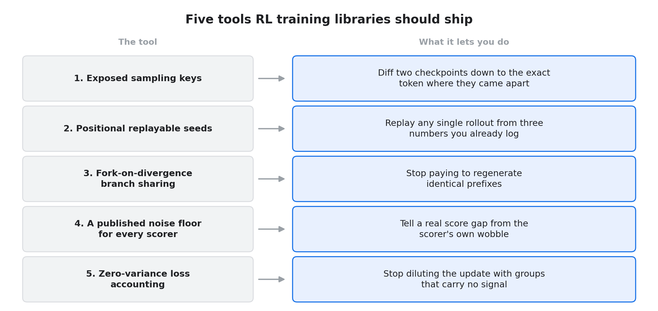
None of these five is a research problem. Each is a small, specific piece of engineering with a mechanism that already has a literature behind it, and the measurements above are what even a cheap prototype of one can show you about your own training run. A library that shipped them would make replay, diffing, and honest signal accounting as ordinary as logging the loss. That is the standard worth asking for.
Riders: every measured number in this piece (the 10.5x reward-model floor spread, the 2.4-point recovery from fixing the loss denominator, the 100-out-of-100 replay result at a fixed batch shape) comes from a single setup, single seed, one model family per measurement. The 2.4-point figure in particular carries p = 0.141 on a paired test and sits inside the roughly 6-point margin a single seed on a 500-question evaluation can resolve at this scale. A different model or task could shift the exact figures, though the mechanisms travel. The GLM-5.2 quote is verified from the model authors’ own public post. Other claims circulating about that training run rest on secondary summaries and are left out of this piece rather than repeated.