What this piece found
- Two training runs that differ in nothing but the random seed can hand you opposite verdicts. Three seeded repeats of one identical comparison produced two decisive raw wins for the same side and one dead heat, with every other source of randomness held bit-for-bit identical between the compared runs. Under the study’s primary scoring rule, which corrects for answer length, the two decisive seeds soften to 60.1% and 68.1% of the match-ups the judge actually decided, and the third crosses over to 43.5%, favoring the other side. Two seeds point one way and one points the other, so the verdict this comparison earns is a near-tie, not two clean wins.
- The four scoring models this piece measured (two used as training rewards, two used as judges) each carry their own measurable wobble, and the spread between the two training-reward scorers, at the extremes of the same protocol and day, is 10.5x. The wobble bound we compute is a worst case: it is set by the noisiest items, so most comparisons sit well inside it, and a typical single comparison is safer than the bound suggests.
- A two-part rule for calling a winner (statistical significance on the pooled evidence AND every seed agreeing in direction) has a cost nobody quotes: going from 3 seeds to 5 left the smallest gap the rule can catch at 3.8 percentage points, the same at 3 seeds as at 5. Seeds 4 and 5 were never run. They exist only inside a simulation, drawn at the noise level the 3 real seeds measured, and inside it the extra seeds bought nothing.
- What does buy resolution is eval questions: for a 3-point gap that all three seeds share, the chance the rule calls it rises from 0.580 at 500 questions to 0.945 at 1,319, computed from each pool’s measured noise.
- The practical order of spending, if you want a comparison you can defend: measure your scorer’s wobble, run 3 seeds, then put every remaining dollar into eval questions, not more seeds.
1. Same recipe, same data, nothing changed but the seed: the verdict didn’t hold
Say you want to know whether a cheaper, noisier way of grading your model’s attempts during training is good enough to swap in for the real thing. You train two copies of the same model, identical except for which grading scheme feeds the training loop, and watch which one comes out ahead. Whichever wins, you’ll trust, and you would expect the same winner if you ran it again with nothing different except the random seed, the number deciding how the model’s weights start out, what order it sees its training examples in, and (as this section will show) which of its own attempts it happens to sample during training.
Here is the full setup, stated up front. Both halves of the comparison are Qwen2.5-1.5B, fine-tuned with a lightweight adapter rather than a full retrain, on Dolly-style instruction-following tasks (“write a note,” “explain X”), trained with GRPO: the model generates several attempts at an answer, each attempt is scored, and the model is nudged toward whichever of its own attempts scored best. One half of each pair trained against the full score handed out by a reward model, GRM-Gemma2-2.6B, a small model trained to rate how good an answer is so that training has something to push toward. The other half trained against a degraded version of that same score: every single training step, half of that score was replaced with pure random noise instead of real feedback. After training, the two final models were graded head-to-head by two independent judge models that never took part in training either run, FsfairX-LLaMA3-RM and RM-Mistral-7B, on 325 held-out questions neither model had seen. Those 325 questions are one fixed set, drawn once and reused at every seed, not a fresh draw per seed. That matters for what follows: when the seeds disagree below, they are disagreeing about the same 325 questions.
We ran this matched pair three times, once per seed. Here is what FsfairX-LLaMA3-RM found when it compared the two final trained models on those 325 held-out questions, picking a winner or a tie for each (a tie meaning the judge’s two scores for that question landed within the judge’s own wobble band, a quantity section 2 measures in full):
| real signal won | half-noise won | tied | |
|---|---|---|---|
| Seed 1 | 185 | 57 | 83 |
| Seed 2 | 106 | 109 | 110 |
| Seed 3 | 202 | 41 | 82 |
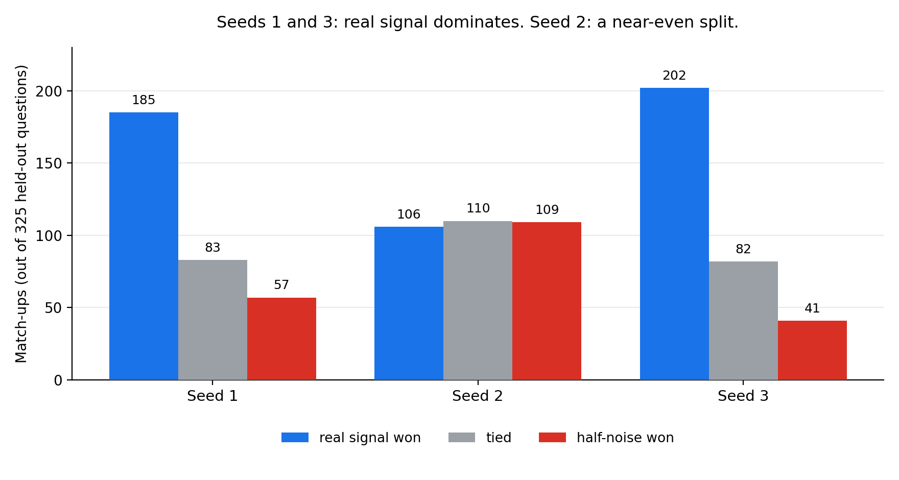
In seed 1 and seed 3, the real signal won decisively. Under pure chance, a split this lopsided has a probability of about 5.8x10^-17 at seed 1 and about 9.5x10^-27 at seed 3, numbers small enough that luck is not a serious candidate explanation. In seed 2, the half-noise model won almost exactly half of the decided matches (109 to 106, with 110 further ties): an even split, not the lopsided pattern the other two seeds showed. A second, independently trained judge, RM-Mistral-7B, scored the same three pairs and saw close to the identical pattern. Seed 1 came out 184 wins to 53 with 88 ties. Seed 2 was an exact 108-108 tie with 109 further ties. Seed 3 came out 200 wins to 36 with 89 ties.
The obvious objection is that the half-noise run in seed 2 simply drew an easier set of practice questions. Normally you could not rule that out: every training run samples its own practice attempts at random, so two runs can differ just because one drew easier material. We closed that door on purpose. Both halves of every pair drew from the exact same underlying randomness, position by position, for the entire run: the same practice questions, sampled the same way, at the same moment, because the rollout sampling itself is driven by a noise stream keyed to the seed, the question, and the training step, never to which half of the pair is training. We checked this directly: at the very first training step, the two halves of each pair produced bit-for-bit identical output. So whatever made seed 2’s pair land even while seeds 1 and 3 landed lopsided, it cannot have been one half drawing easier material: within every pair, both halves drew identical material. The only ingredient that changes from one pair to the next is the seed itself, the starting weights and the data order it sets. That is what makes the dead heat a fact about the seed, not about the reward signals being compared.
All three readings report what the judge actually scored. Seed 2’s dead heat is not a data error: on the recorded votes it is a dead heat by any reading. Whether some hair-thin true preference hides beneath it is exactly what a single reading cannot resolve, as section 2 will make precise. What stands is the contrast: two seeds produced decisive splits, one produced a dead heat, and nothing but the seed changed.
That a seed can swing a reinforcement-learning result this much is not news by itself. A well-known 2018 study (Henderson et al., “Deep Reinforcement Learning that Matters”) found that changing nothing but the seed shifted results as much as changing the algorithm did. What is narrower here is that because both halves of each pair shared identical dice, “one run got luckier material” is ruled out as the explanation. Most seed-variance findings cannot rule that out. This one can.
Both judges’ raw preference tracks answer length to some degree. Longer answers score a little higher independent of whether they are actually better. Statisticians handle a confound like this by residualizing it out: fit the relationship between length and score, then look at what is left over once that relationship is subtracted. Do that here, and length turns out to explain a little over a third of the variation in these judges’ raw scores (an r-squared of 0.37 for one judge and 0.38 for the other, across the same 975 pairwise comparisons). The length-corrected reading is this study’s primary one, fixed in advance. The raw counts in the table above are its secondary reading, and they are the ones the eye goes to first, which is why both belong on the page.
Here is the same comparison read both ways, under FsfairX-LLaMA3-RM, as the real signal’s share of the match-ups the judge actually decided (ties excluded from the share, listed alongside):
| Seed | Raw win share | Length-corrected win share | Length-corrected counts (real / half-noise / tied) |
|---|---|---|---|
| 1 | 76.4% | 60.1% | 131 / 87 / 107 |
| 2 | 49.3% | 43.5% | 83 / 108 / 134 |
| 3 | 83.1% | 68.1% | 145 / 68 / 112 |
RM-Mistral-7B, scoring the same pairs, gives 58.0%, 43.7% and 68.6%. Correcting for length costs the real signal 16.4 points of win share at seed 1 and 15.1 at seed 3, which stay clearly on its side, and pushes seed 2 across the even line to 6.5 points on the half-noise side under FsfairX-LLaMA3-RM and 6.3 under RM-Mistral-7B. Seed 2’s corrected lean reaches p = 0.08 under FsfairX-LLaMA3-RM and p = 0.09 under RM-Mistral-7B, so it is a lean and not a demonstrated reversal.
The bar fixed in advance for this comparison: every seed’s sign must agree, and most seeds must clear significance individually. It is a different rule from section 3’s two-part rule of section 3, which pools first and requires unanimity on top. On the length-corrected reading, 2 of the 3 seeds clear significance individually but the signs do not agree, so the bar does not clear and the verdict is a near-tie. That sign disagreement is the thing to carry forward: seeds 1 and 3 land positive, seed 2 lands negative, on the same recipe and the same data, with nothing changed but the seed.
If a comparison this controlled can change its verdict on the seed alone, then any published “A beat B” carries a hidden question: was that A, or was that A’s seed? The rest of this piece puts numbers on the answer.
2. Every scorer wobbles, and different scorers wobble very differently
Section 1 showed what the seed alone can do to a verdict. There is a second instrument in that comparison that can move a verdict just as much: the scoring model doing the judging.
Say you have two candidate answers to the same question, and you are using a reward model to pick the better one. It scores one of them a hair higher. You ship that one. Now score the exact same pair of answers again: same text, not one character changed, just a different batch of other stuff sitting around it in memory. The number moves. How far it can move, for reasons that have nothing to do with which answer is actually better, is what the rest of this section measures.
Which of those two scores do you believe? You cannot tell, not without a third piece of information: how much this particular model’s score for this particular kind of text wobbles on its own, for reasons that have nothing to do with quality. Call that number the noise floor. Score two things and get a gap smaller than the floor, and you do not actually know which one is better. You have measured the model’s own wobble, not a preference.
Think of it like a ruler that is slightly warped. Measure the same board twice and you will read two slightly different lengths, not because the board changed but because the ruler itself has some give. The noise floor is how much give this particular ruler has, and until you have measured that give, you cannot tell a real difference in length from the ruler just flexing.
Here is what that looks like on one real item: one item, scored repeatedly under varying batch company. One held-out instruction from this study asked “Why did the Allies invade Normandy during world war 2?” The base model’s greedy response opened “The Allied invasion of Normandy, codenamed Operation Overlord, was part of the D-Day landings in June 1944. It was a massive operation to liberate Western Europe from Nazi occupation and pave the way for the eventual defeat of Nazi Germany. The success of this campaign marked a turning point in World War II and led to the liberation of Paris and other key cities by July 1944.” GRM-Gemma2-2.6B scored that exact (instruction, response) pair 20 times: once alone, and 19 more times embedded in 8-item batches, at positions 0, 3, and 7, with a fresh random draw of filler items each time. The first few scores give the flavor: 2.6035 alone, then 2.6094, 2.6055, 2.6055, 2.5957 across the first four embedded contexts. Across all 20, the highest score was 2.6152 and the lowest 2.5957, a spread of 0.0195 for one unchanged answer. That is half again larger than the 0.0131 p95 jitter the original floor protocol measured across all 64 items. The two protocols also differ: the original floor run reused one fixed filler batch, while the re-scoring drew fresh fillers each context. A wider spread under fresh fillers is the direction that difference predicts, though one item cannot establish it. (These 20 scores come from a later re-scoring pass over the same item, by the same scoring model, not the original run behind the floor table below, which kept only summary statistics and discarded its raw repeated scores, and the re-scoring pass used 20 contexts at positions 0, 3, and 7 with fresh fillers, while the floor protocol below uses 5 fixed contexts at positions 0 through 3.)
Measuring the floor itself takes one protocol, run once. Score a fixed set of items alone (one item per batch), then score each of those same items again while it sits at a different position inside a small batch of otherwise unrelated filler items, four positions in all. Nothing about the target item’s own text changes across these five scores, only what is sitting next to it in the batch, and where. Per item, jitter is the highest of those five scores minus the lowest. Pool every item’s jitter into one list, take the 95th percentile of that list (the value 95% of items’ wobble falls at or under, so a couple of freak outliers cannot inflate it), multiply by 3, and that is the floor: labeled EPS in the table below. The 3 is a safety multiplier fixed when the protocol was designed: p95 jitter is one draw’s spread, and tripling it builds in headroom before treating a gap as real. Any score gap smaller than EPS is a tie, not a verdict.
We ran that check against four scoring models people actually use in this kind of pipeline (two trained to hand out a reward during RL training, two used afterward as judges), on the same 64 (question, response) pairs, base-model outputs to Dolly-style instructions:
| Scoring model | Used as | Noise floor (EPS) | p95 jitter |
|---|---|---|---|
| GRM-Gemma2-2.6B | training reward | 0.0393 | 0.0131 |
| Skywork-Reward-V2-Qwen3-8B | training reward | 0.415 | 0.138 |
| FsfairX-LLaMA3-RM | judge | 0.274 | 0.0914 |
| RM-Mistral-7B | judge | 0.281 | 0.0938 |
(Skywork-Reward-V2-Qwen3-8B is shortened to Skywork-8B for the rest of this piece and in the figure below.)
The two scorers used as judges in section 1 sit in the middle of this table, at 0.274 and 0.281, nearly identical to each other. The 10.5x spread is between the two training-reward scorers at the extremes. What matters for section 1 is the judges’ own floors: a per-question score gap inside 0.274 is inside the primary judge’s own wobble.
Repeatability is not the only thing you would want to know about these scorers, and the second thing cuts across the first. A separate ranking run in this project scored these same models on how well they tell a good finished answer from a bad one, on two kinds of question: factoid trivia and science questions. Skywork-8B, the scorer with the widest floor here, came first on both, capturing 77.90% of the distance from a coin flip to a perfect grader on the trivia questions and 58.48% on the science ones. GRM-Gemma2-2.6B, the steadiest scorer here, captured 59.77% and 32.54%. Section 1’s two judges land in between: FsfairX-LLaMA3-RM at 74.99% and 45.17%, RM-Mistral-7B at 62.56% and 34.54%, which leaves the second judge about 15 points behind Skywork-8B on trivia and about 24 points behind it on science. Those per-question-type figures are the ranking’s primary reading. Collapsing them into a single average (68.19% for Skywork-8B against 46.16% for GRM-Gemma2-2.6B) hides exactly the task-to-task difference the ranking exists to show, which is why the ranking carries the average as a summary column and not as its result. The point for this section survives either reading: the best judge in this set is the least repeatable scorer in it. Those are two different properties, measured two different ways, and a ranking on one is not evidence about the other.
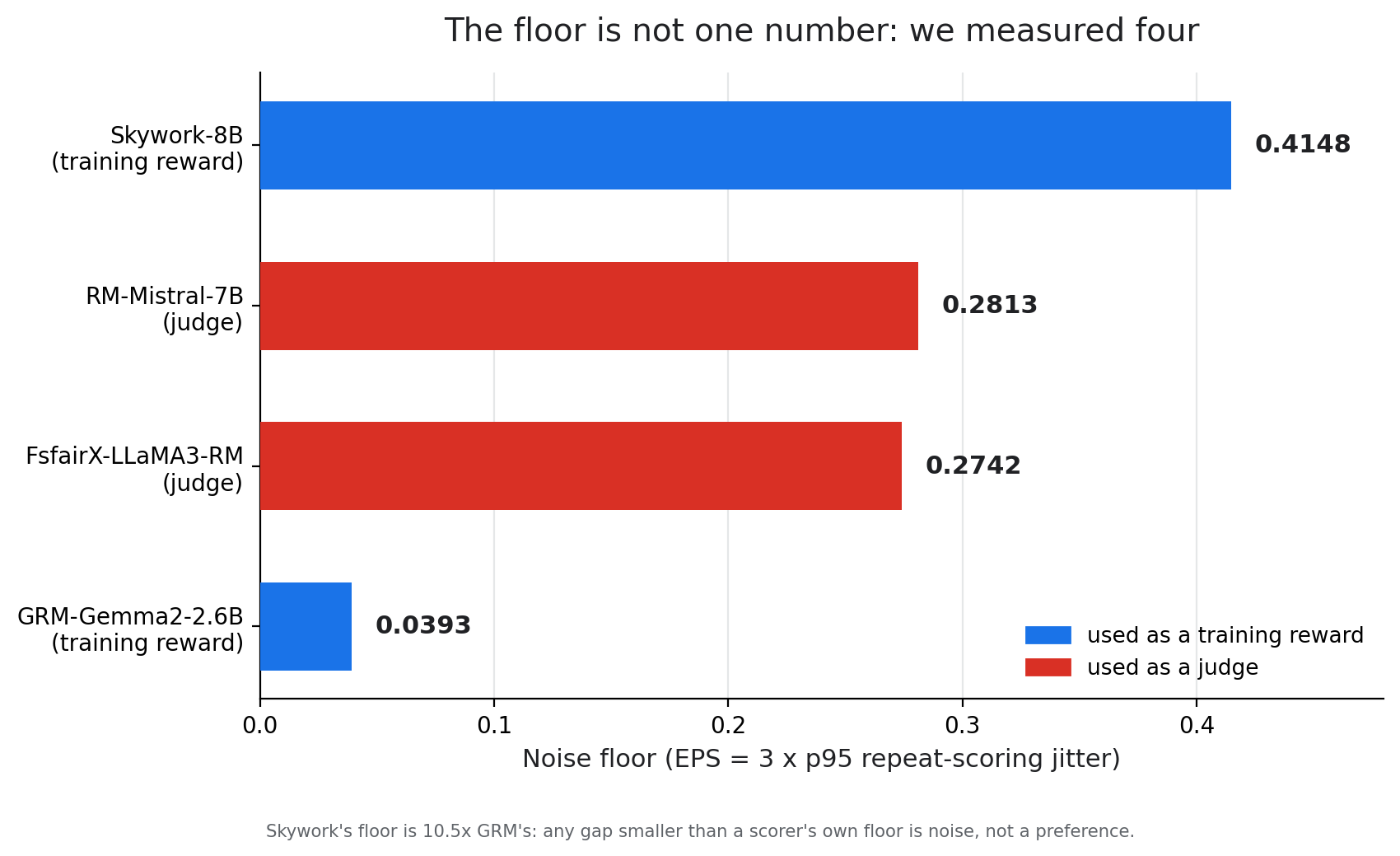
Same protocol, same 64 items, same day: the whole table was measured once per scorer, on that one day. A partial re-run later, on different hardware, landed within about 20% of these figures. The floors span a 10.5x range: Skywork wobbles ten times harder than GRM. A tenth of a point separates two answers under GRM and that gap might be real. The same tenth under Skywork is pure wobble. There is no single noise floor for reward models in general. There is a floor for a specific model, on a specific kind of text, and you do not know yours until you measure it.
Floors are regime-specific, not model-specific, and that cuts against reusing anyone else’s number, including our own from a different task. The same GRM model, measured on short trivia-style answers instead of the instruction-response text above, floors at 0.0636 instead of 0.0393, a measured +62%. That move is far outside the roughly 20% spread the partial re-run showed, so it is a change of regime and not the instrument drifting. Skywork-8B, measured the same way, moves from 0.415 to 0.462, a change of 11%, and 11% sits inside that re-run spread. Whether Skywork’s floor really moves with the kind of text is not settled by these two readings. Same model, different kind of text, different wobble, at least where the measurement can resolve it. Measure yours. Do not borrow ours.
One caution on reading that floor: it is deliberately a worst case. The 95th percentile is set by the noisiest items, and most pairs of outputs sit far inside it, so the floor tells you when to distrust a small gap, not how noisy a typical comparison actually is.
That worst case is the band section 1 used to call a match-up a tie, and it is borrowed twice over. It was measured on the base model’s answers, not on the answers the two trained models in section 1 actually produced, which is the reuse this section has just argued against. And it is a bound built around the noisiest items, three times their jitter, then applied as the threshold for every individual question. Both choices push the same way. They widen the tie column and shrink the pool of match-ups that get decided at all.
Narrowing the band moves those counts, so here is where they move to. Recounting the same stored judge scores at a narrower band, first with the safety multiplier dropped (leaving the 95th-percentile jitter itself, 0.0914 for FsfairX-LLaMA3-RM) and then with the band removed entirely, gives seed 2 under that judge:
| Tie band | Seed 2, length-corrected | Seed 2, raw |
|---|---|---|
| 0.274, 3x jitter, the band used above | 83 / 108, 43.5%, p = 0.08 | 106 / 109, 49.3% |
| 0.0914, multiplier dropped | 118 / 150, 44.0%, p = 0.06 | 146 / 134, 52.1% |
| 0, identical scores only | 144 / 176, 45.0%, p = 0.08 | 166 / 151, 52.4% |
The direction the primary reading gives is stable: seed 2 stays on the half-noise side at every band, under both judges. The raw reading is the fragile one, sitting a hair below even at the wide band and a hair above it at the two narrower ones, so which side its raw score lands on depends on where the band is drawn. What no band changes is the distance between the seeds. On that raw reading, seed 2 stays within 2.4 points of even at all three settings, while seeds 1 and 3 stay between 70.0% and 83.1%.
3. The two-part rule for calling a winner, and a dry run of it
A single seed’s verdict can be the wrong one to trust, so no single reading gets to call a winner here. A comparison counts as a win only when both parts of the following rule hold.
Section 1’s experiment and the material from here through section 5 come from two different studies. This section, and sections 4 and 5, move to a separate study on GSM8K (grade-school arithmetic word problems), training the same Qwen2.5-1.5B model family across nine training runs, each repeated at three seeds, and comparing pairs of those runs to each other with an automatic right-or-wrong checker instead of a judge model.
First, we pool the evidence from every seed together and run one significance test on the combined counts: does the combined pattern look too unlikely to be chance? Second, we check that every individual seed, taken on its own, points the same direction, not just most of them. The comparison counts as a win only when pooled significance holds AND every seed agrees on direction. Call that the two-part rule.
Why does agreement across every seed earn a place in the rule, on top of a good pooled number? Because the two halves ask different questions. The pooled test asks how many individual questions lean one way once every seed’s verdicts are combined, and it can return a very confident answer while one entire run points the other way. Section 1’s comparison has exactly that shape. Pooled across its 3 seeds on the raw reading it reaches p = 7.4x10^-19, about as decisive as a significance test gets, and seed 2 still lands on the opposite side from the other two. The unanimity half is what refuses to call that a win. It asks whether each run, taken whole, agrees, which is the question you are actually asking when what you want to know is whether running the experiment again would hand you the same winner.
Adding seeds pulls the rule’s two halves in opposite directions. The pooled half gets easier to satisfy as seeds are added: more seeds means more combined evidence, and a significance test with more evidence to work with is more sensitive, the same way a poll of a thousand people gives a tighter estimate than a poll of ten. The unanimity half gets harder as seeds are added. Suppose, purely to run the arithmetic, that a given seed has a 0.8 chance of landing on the correct side of some small, real effect. The chance two seeds both land there is 0.8 x 0.8, or 0.8^2 = 0.64. Add a third seed and it drops to 0.8^3 = 0.512. Add two more and it drops further, to 0.8^5 = 0.328. In general, if a single seed’s chance of landing on the correct side is p, the chance every one of n seeds lands there is:
P(all n seeds agree) = p^n
a number that shrinks every time n grows, for any p below 1.
Two terms recur from here on. The 22.6% noise level: across 12 different pairwise comparisons in this same GSM8K study, on average 22.6% of the 500 questions get a different right-or-wrong verdict depending on which of the pair’s two checkpoints answers them, at a given seed. That is the base level of question-to-question noise the two-part rule has to see through. The smallest catchable gap: the smallest true difference between two things being compared that this rule can be trusted to catch, meaning call both significant and unanimous, at least 80% of the time, given that measured noise level.
To find the smallest true gap this rule can actually be trusted to catch, we ran a Monte Carlo simulation, and one simulated dataset in it is a pretend rerun of the whole comparison. It has the same shape as the real thing, 500 questions times 3 seeds. Each question, under each seed, either casts a vote or goes silent, silent at the same rate the real runs measured (the 22.6% noise level just defined is the share of questions that cast a vote at all). A cast vote goes to the truly better side slightly more often than half, by exactly enough that the built-in advantage equals the gap size being tested. Apply the two-part rule to one pretend rerun exactly as to real data, and it either calls the winner or stays silent. Repeat many thousands of times at each candidate gap size, and the share of pretend reruns where the rule calls the winner is that gap’s catch rate. Before running that at scale, here is the rule worked through on one real comparison from this project, seed by seed.
One training run in this study, the full-reward-model configuration, trained against a dense GRM-Gemma2-2.6B reward signal (its complete score, every training step, not the fair-accounting checker or tie-break signals section 4 turns to), saw its accuracy peak partway through training and then decline, a known failure pattern in reinforcement-learning fine-tuning where a model overfits its own reward signal. We compare that run’s own peak checkpoint against its own final checkpoint, seed by seed, on the same fixed 500-question pool:
| Seed | Peak checkpoint accuracy | Final checkpoint accuracy | Per-seed gap | Direction |
|---|---|---|---|---|
| 1 | 60.8% | 56.4% | +4.4 pp | peak ahead |
| 2 | 62.0% | 56.4% | +5.6 pp | peak ahead |
| 3 | 62.2% | 56.8% | +5.4 pp | peak ahead |
(Gaps above, and elsewhere in this piece, are in percentage points, pp for short.)
All three seeds point the same way: the peak checkpoint ahead. That clears the unanimity half of the rule. The pooled test works per question, not per seed. For each of the 500 questions, take the three seeds’ verdicts and keep the majority: if two or three seeds agree on a direction, that question casts one vote that way. If the seeds split with no majority, the question abstains. On this comparison, 190 of the 500 questions cast a vote: 114 for the peak checkpoint, 76 for the final one. An exact two-sided binomial test on those 190 votes gives p = 0.0071. Note what this count is not: it is not any single seed’s flip rate, and it will not match the per-seed nets in the table above, because the majority vote filters differently than any one seed does. Both halves of the rule hold, so this comparison counts as a called win.
4. Simulate a fourth and a fifth seed, and the rule spends them on nothing
The Monte Carlo simulation described above, run at this project’s own measured 22.6% noise level, gives the smallest catchable gap at 3 seeds and at 5: 3.83 points at 3 seeds, 3.79 at 5. Essentially flat. Drop the unanimity requirement and score on pooled significance alone, and the same simulation gives 3.44 points at 3 seeds and 2.67 at 5: seeds do real work there. The unanimity requirement is what erases it.
The 5-seed figure is a simulated one. Three seeds is what these runs actually paid for, and seeds 4 and 5 exist only inside the Monte Carlo, drawn at the noise level the 3 real seeds measured. So the claim here is not “we bought two more seeds and watched them do nothing.” It is that at this measured noise level, the rule’s own arithmetic says two more seeds would do nothing, which is the cheaper way to find that out and the reason to find it out before spending.
Section 3’s arithmetic explains why. The pooled test does get a little more sensitive with each seed added, because more seeds means more evidence accumulating toward the significance threshold. But the chance that every one of those seeds independently lands on the correct side keeps shrinking as more are added, for the same reason the worked equation showed a moment ago: a fixed per-seed chance, raised to a growing power, only gets smaller. At this project’s own measured noise level, across the seed counts that actually matter in practice, the two effects trade off closely enough that buying two more seeds bought nothing.
That claim has a boundary worth marking. The arithmetic above is about catching a gap that every seed shares, and for that job the extra seeds trade off against themselves. Whether the seeds share a gap at all is a different question, and it is the one section 1 answered: no eval pool of any size would have revealed that seed 2 landed even, because only running a second and a third seed could reveal it.
A second comparison from the same study, alongside the peak-versus-final case worked through in section 3, makes “called” against “stays undecided” concrete. This one sets the fair-accounting checker configuration against the localized tie-break configuration, each read at its own converged checkpoint, on the same 3 seeds and the same 500-question pool.
Both sides need naming precisely, because a companion piece runs what sounds like the same comparison and gets a different answer. The fair-accounting checker configuration trains on the automatic checker’s right-or-wrong signal alone, with no reward model anywhere in the loop, and with one correction applied: when a question’s whole group of sampled attempts comes back all-right or all-wrong, that group contributes no signal, and this configuration also drops it from the count it averages over, instead of dividing by it. The localized tie-break configuration trains on that same checker signal with a reward model stepping in to rank attempts the checker graded identically. There is no plain, uncorrected checker configuration in this 3-seed set of runs, so nothing below compares against one.
The two configurations stopped training at different step counts for two of the three seeds: seed 1 finishes both configurations at a common step 150, while seeds 2 and 3 finish the fair-accounting checker configuration at step 250 against the localized tie-break configuration’s step 150. What gets compared, seed by seed, is each configuration’s own finishing point, not a shared step number across every seed.
| Comparison | Votes for the fair-accounting checker | Votes for the localized tie-break | Votes cast (of 500) | Pooled significance | All 3 seeds agree on direction? | Verdict |
|---|---|---|---|---|---|---|
| the fair-accounting checker configuration vs. the localized tie-break configuration, each at its own converged checkpoint | 96 | 78 | 174 | p = 0.197 | Yes | Undecided |
This comparison is not a failure of unanimity. All three seeds agreed, every time, on direction, and the direction is the fair-accounting checker a hair ahead, by 0.8, 2.2 and 2.2 points across the three seeds. What failed was the pooled test: gaps that small, against the 22.6% noise level this rule has to see through, do not move 174 votes far enough from an even split to clear significance.
Two things about that result are worth stating plainly rather than filing as a success.
The first is what this comparison does and does not settle about the tie-break. The companion piece on reward shopping reports the localized tie-break winning 40 questions the checker got wrong while losing 15 the checker got right, a gap that would come up by chance about 1 time in 1,000. That is a different run read a different way. It is a single seed, on a separate pair of training runs, trained for fewer steps, read at one fixed checkpoint, with a paired test on that seed alone, and the checker on the other side of it there is a plain one, without the all-same-group accounting correction described above. The comparison in this section is 3 seeds, each side read at its own converged checkpoint, pooled by per-question majority vote across the seeds and then tested. Neither reading is the other’s replication, and nothing in either one explains why they land on opposite sides. What can be said is the thing this piece opened with: one seed at one checkpoint handed the tie-break a clear win, 3 seeds each at their own converged checkpoint did not, and the difference between those two answers is not by itself a fact about the tie-break.
The second is the rule grading its own homework. This comparison was picked in advance as the one where the two configurations were expected to be indistinguishable, so “undecided” is the answer the setup was looking for, and a rule returning the expected answer on a case chosen for it has not thereby been shown to tell a real tie from a gap it merely cannot see. The prediction was also not right in detail: it said the three seeds’ directions would split, and they did not, they agreed. What the rule demonstrates here is narrower than “it correctly stays undecided.” It is that under this rule, a consistent 0.8 to 2.2 point gap at 3 seeds and 500 questions does not clear the rule, which is the same fact section 5 turns into a cost table.
5. Eval questions sharpen the verdict. Here is what that costs.
If buying more seeds under this rule buys almost nothing, what does? The 22.6% noise level driving the arithmetic above comes from evaluating each checkpoint on a 500-question pool. Shrink that noise instead, by evaluating on more questions per seed, and both halves of the rule improve together instead of trading off, because a bigger eval pool lowers the noise level itself rather than just adding more repeats at the same noise level.
Holding seed count fixed at 3 and only growing the eval pool, for a 3-point true gap shared by all three seeds:
| Eval pool size (3 seeds) | Chance the rule calls a 3-point gap |
|---|---|
| 500 | 0.580 |
| 750 | 0.774 |
| 1,000 | 0.864 |
| 1,319 (full GSM8K test split) | 0.945 |
| 2,000 (extended pool) | 0.990 |
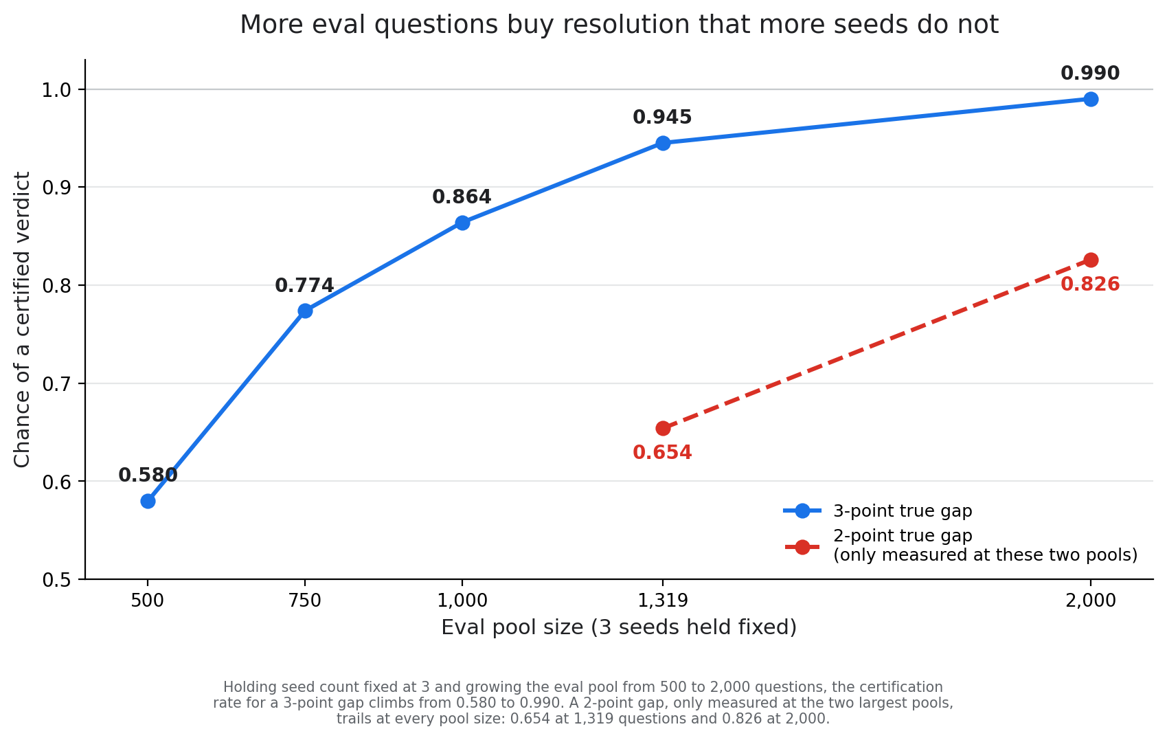
A 2-point gap needs more questions than a 3-point gap to reach the same confidence, because a smaller true effect is harder to separate from noise at any fixed pool size. The chance of a called verdict on a 2-point gap was only computed at the two largest pools: 0.654 at the full 1,319-question test split, 0.826 at the extended 2,000-question pool. Both the 1,319-question and 2,000-question rows above started life as predictions, made before either pool existed: the pre-registered simulation projected 0.943 (3-point gap) and 0.663 (2-point gap) at 1,319 questions, and 0.990 and 0.833 at 2,000. Both pools were then built, verified never used in training, and each pool’s own per-question discordance was measured directly: 0.2223 at the 1,319-question test split, 0.2256 at the 2,000-question pool. The chance of a call was then recomputed from that measured noise, the same Monte Carlo procedure run at each pool’s own measured discordance rather than at the pre-registered projection: 0.945 and 0.654 at 1,319, and 0.990 and 0.826 at 2,000.
Every number in that table rests on one assumption about how seeds differ. The simulation treats the true gap as a single fixed quantity every seed shares, so that all disagreement between seeds is sampling noise, the kind more questions can average away. The judged comparison this piece opened with is a warning that reality is not always so obliging: there, the pooled raw-score test put the two training runs apart at odds of about one in 10^18, and one of the three seeds still read a dead heat. Under a single shared gap that combination is essentially impossible. Some of what separates seeds in that regime is not noise at any pool size. The seeds themselves differ. So read the cost table as what questions can fix, which is noise. Where seeds truly differ, no eval pool restores unanimity, and finding that out is precisely what running more than one seed is for.
Growing the eval pool shrinks the smallest catchable gap in a way growing the seed count, under this exact rule, does not.
The same arithmetic applies when the checker is not automatic. Most training decisions that matter in practice have no right-or-wrong answer key, so an AI judge’s preference substitutes for the checker’s verdict, and the simulation runs exactly as before, mechanically unchanged, except now a “verdict” means which of two outputs the judge preferred rather than which one matched an answer key. This is the same 3-seed judged comparison from section 1, on that one shared 325-question pool (FsfairX-LLaMA3-RM and RM-Mistral-7B judging the real-signal versus half-noise pair), reanalyzed here for its own catchable gap rather than its raw win counts (this reanalysis applies section 3’s pooled-and-unanimous two-part rule, not section 1’s own pre-set bar for calling a clean win).
Run the rule on that comparison and it stays silent, under either judge and under either scoring column. The pooled half passes easily, at p = 0.0079 on the primary length-corrected reading and p = 7.4x10^-19 on the raw one. The unanimity half fails, because seed 2 never joins the other two: under RM-Mistral-7B’s raw scores it lands on an exact 108-108 split, and under the other three readings it points the other way. Section 1’s opening comparison, the one this piece starts from, is a comparison this piece’s own rule declines to call. That is the rule working as intended rather than a hole in it. After 3 seeds and 975 judged match-ups, there is no called winner between a real reward signal and one half-replaced with noise.
Judged comparisons resolve to a preference far more often than accuracy checks resolve to a clear right or wrong: pooling 12 readings of this single comparison (two judges times two scoring columns, raw and length-corrected, times three seeds), the measured per-question disagreement rate averages 67.2%, about three times the 22.6% average across the GSM8K ladder’s 12 separate pairwise comparisons in section 3. Combined with a smaller pool (325 questions rather than 500), that pushes the smallest catchable gap up: at the 3 real seeds this comparison actually used, it is 8.68 points of judged win share, more than twice GSM8K’s 3.8 accuracy points. The two are different units and not two measurements of one thing: 8.68 points is a share of the match-ups a judge decided, and 3.8 points is a difference in the fraction of arithmetic questions answered correctly. Each is what the same rule needs before it will call a winner in that setting. Running the same simulation forward to a hypothetical fifth seed, never actually collected, projects a smaller drop to 8.17 points, the same near-flat pattern as the GSM8K accuracy ladder, just less perfectly flat here. A bigger prompt pool would shrink it the same way growing the GSM8K pool did: it is the lever that works, not more seeds.
6. Checklist for your training
This list is written to stand alone. If someone hands you only this section, it is the whole procedure.
- Measure your scorer’s wobble before trusting any gap it reports. Take about 60 held-out items. Score each one alone, then four more times at different positions inside a small batch of unrelated filler items, five scores per item in all. Per item, subtract the lowest of the five from the highest. Take the 95th percentile of those spreads across items and multiply it by 3. That is your scorer’s noise floor, on its own scale. Any score gap smaller than the floor is a tie, not a preference. Floors differed by 10.5x across the four scorers we measured and moved with the kind of text being scored, so measure your own. Do not borrow anyone’s, including ours.
- Run 3 seeds, not 1 and not 5. Repeat the whole comparison three times with nothing changed but the random seed. One seed alone can hand you a dead heat where two others show a landslide, which is exactly what happened here. Past three, the gains cancel: each added seed sharpens the pooled evidence and adds one more chance for a run to point the other way, and at our measured noise the smallest gap the rule could catch was the same at 5 seeds as at 3.
- Then put every remaining dollar into eval questions, not more seeds. A bigger question pool shrinks every seed’s own noise and keeps paying. At our noise level, growing the pool from 500 to 1,319 questions took the chance of calling a real 3-point gap from 0.58 to 0.95. Two extra seeds took it nowhere.
- Call a winner only when both parts hold. Pool the seeds question by question: each question’s majority verdict across the three seeds is one vote, and an exact two-sided binomial test on those votes must come back significant. Separately, every seed’s own overall direction must agree. Both together are a win. Anything else, report the smallest gap your setup could have caught instead of declaring a winner. At our scale that floor was 3.8 accuracy points on the checkable task and 8.7 points of judged win share on the open-ended one.
Where each number comes from, for anyone who wants the full derivations: the wobble protocol and the floors are section 2, the seed arithmetic is sections 3 and 4, and the question-pool chances are section 5.
Every number in this piece comes from one model family (Qwen2.5-1.5B), fine-tuned with lightweight adapters rather than full retrains, at toy scale (100-step runs, 500 to 2,000-question eval pools). Each instrument was measured on one task family: section 1 and 2’s judge-based numbers on Dolly-style instruction tasks, sections 3 through 5’s two-part-rule numbers on GSM8K arithmetic problems. A different model, a longer run, or a different task would shift the exact figures. The method, in every section, travels.